reading tsg files
- 5 minutes read - 888 wordsGood Afternoon Spectroscopists,
I though someone might be interested in using pytsg to process hyperspectral data. For this example we are going to use this dataset provided by CSIRO under a CC4 licence collected for the C3DMM project
In this post we will use of PLS to predict Fe grade from the spectra.
Let us start by installing the libraries that we are going to need. You can use the tsg file reader that I developed here or you can write your own…
pip install pip install pytsg
pip install matplotlib numpy scikit-learn openpyxl
Once we have the required libraries we are going to download the data that we need for our quick demonstration.
import json
import urllib.parse
import urllib.request
from pathlib import Path

# we are going to use the swagger api to get the files from here programatically this first call here is to list all the available files
url =  'https://data.csiro.au/dap/ws/v2/collections/44783v1/data'
with urllib.request.urlopen( url ) as response:
    response_text = response.read()
# the variable response_text is returned as a json package we are going to parse
# it with the python json library
c3dmm_files = json.loads(response_text)
base_dir = Path('data/')

# here is a list of the target files that we are going to need to
# do this experiment
target_files = ['RC_data.bip','RC_data.tsg','Rocklea_Assay_MMX.xlsx']

# loop over each of the files in the json
# if you've already downloaded them then we won't download the files again.
for i in c3dmm_files['file']:
    # pathlib makes path handling simple I prefer it generally over the os library
    fname = Path(i['filename'])
    url = i['link']['href']
    # if the file names is in the list of target files let's download
    if fname.name in target_files:
        outfile = base_dir.joinpath(fname)
        # check if the folder exists if not make it
        if not outfile.parents[0].exists():
            outfile.parent.mkdir(parents=True,exist_ok=True)
        # check if the file exists if it does then don't download
        if not outfile.exists():
            # downlaod the file
            with urllib.request.urlopen( url ) as response:
                response = response.read()
                with open(outfile,'wb') as file:
                    file.write(response)
Now that the data is downloaded it is a simple process to import the required spectra.
import pandas as pd
from pytsg.parse_tsg import read_tsg_bip_pair

assay_path = base_dir.joinpath('drill hole data/drillcore geochem/Rocklea_Assay_MMX.xlsx')
assay_data = pd.read_excel(assay_path)
tsg_file = base_dir.joinpath('drill hole data/RC_hyperspectral_geochem/RC_data.tsg')
bip_file = base_dir.joinpath('drill hole data/RC_hyperspectral_geochem/RC_data.bip')
nir = read_tsg_bip_pair(tsg_file, bip_file,'nir')
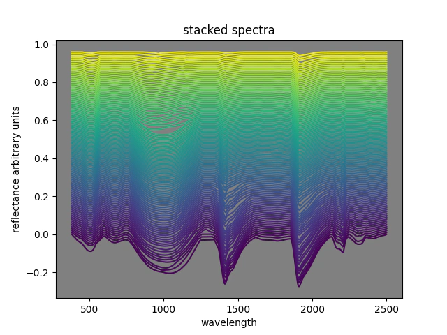
Obviously we would like to have a pretty picture.

To make your own pretty picture run the code below.
# we are going to make a nice looking plot
# to get that to work we will use the convex hull of the spectra
# and then add a little to each spectra so that it looks pretty
from matplotlib import cm
steps = 100
cmap = cm.get_cmap('viridis',steps)
from scipy import spatial
n_spectra = nir.spectra.shape[0]
tmp_spec = []
for i in range(steps):
    spec = nir.spectra[i,:]
    # set up the x and y to calculate the convex hull on
    spec_xy = np.vstack([nir.wavelength,spec]).T
    # calculate the convex hull
    chull = spatial.ConvexHull(spec_xy)
    # sort the verticies then interpolate
    # the data across each of the wavelengths
    sort_v = np.sort(chull.vertices)
    hull = np.interp(np.arange(n_spectra),sort_v,spec[sort_v])
    # this is the remove any spectra where the hull is not calculated perfectly
    if not np.any(spec-hull >0):
        tmp_spec.append(spec-hull)

spec = np.vstack(tmp_spec)
# sorting the spectra in this case orders them very nicely
spec = np.sort(spec,0)

ax = plt.axes()
ax.set_facecolor("grey")
for i in range(spec.shape[0]):
    ax.plot(nir.wavelength,spec[i,:]+(i/100), color=cmap(i))
plt.title('stacked spectra')
plt.ylabel('reflectance arbitrary units')
plt.xlabel('wavelength')
plt.show()
If we were trying to get an estimate of the grade of the material we could use a handheld hyperspectral scanner and apply the model that we have generated here (I am not responsible for the outcomes of this, you are on your own).
Stepping through the process below we will generate a model.
# before we can get anywhere we need to extract the HoleID from the tsg scalars.
# extract the tsg final mask we need this to remove problematic spectra
final_mask = nir.scalars['Final Mask']>0

borehole_info = nir.scalars[['Borehole ID', 'Depth from', 'Depth to']]
idx_borehole = borehole_info['Depth from']<0
borehole_info.loc[idx_borehole,['Depth from','Depth to']] = None
borehole_info.rename(columns={'Borehole ID':'Hole_ID'},inplace=True)

# step through a few qa steps
# merge this data to the assay data that we have imported a while back
merged_assay = pd.merge(borehole_info,assay_data,how='left')
idx_paired = merged_assay.Hole_ID !=''
# ensure that x and y are finite
idx_finite_x = np.all(np.isfinite(nir.spectra[0,:,:]),1)
idx_finite_y = np.isfinite(merged_assay.Fe)
# in this case if fe is 0 it is in error
idx_pos_y = merged_assay.Fe>0
# aggregate all the steps together
idx_final = idx_paired & final_mask & idx_finite_x & idx_finite_y & idx_pos_y
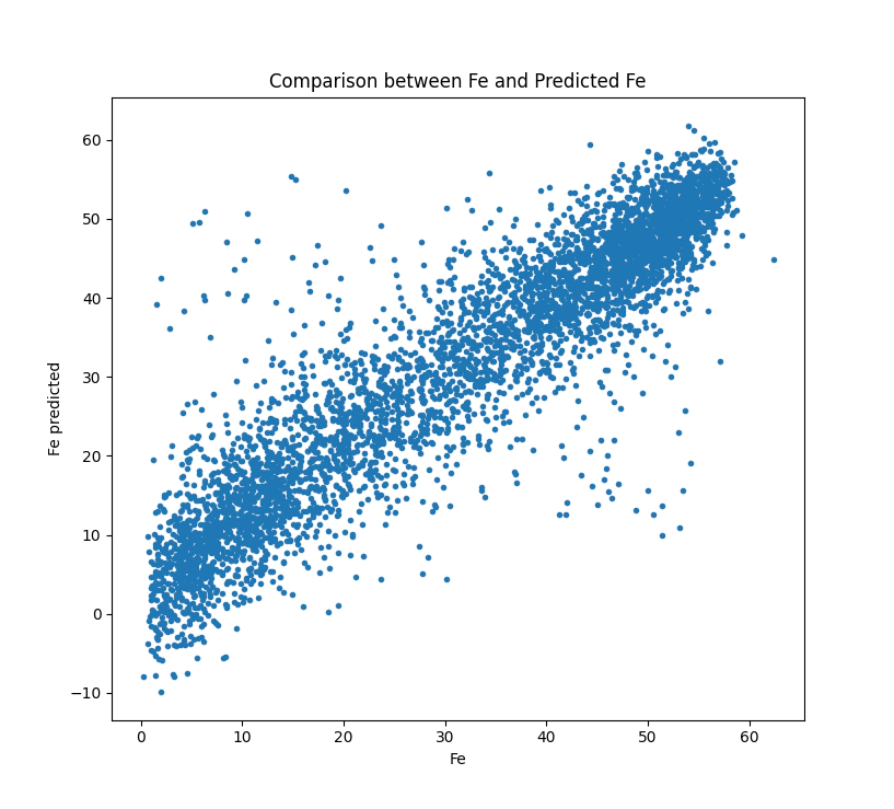
Finally we have done all the qa and data manipulation to get to the point where we can assess the performance of the model.
It should be noted that the vast majority of the code and the effort involved in getting to a prediction is setting up the data to run the regression.
But once we are ready to regress it is a simple process.
from sklearn.model_selection import train_test_split
from sklearn.metrics import r2_score, mean_squared_error
# actually make a model
X_train, x_test, Y_train, y_test = train_test_split(nir.spectra[0,idx_final,:], merged_assay[idx_final].Fe, test_size=0.3)
model = PLSRegression(30).fit(X_train, Y_train)

r2 = 'R2: ' + str(np.round(r2_score(y_test, model.predict(x_test)),2))
rmse = 'RMSE: ' + str(np.round(mean_squared_error(y_test, model.predict(x_test), squared=False),2))
# make a plot
plt.plot(y_test, model.predict(x_test),'.')
plt.plot(range(60), range(60))
plt.xlabel('Fe')
plt.ylabel('Fe predicted')
plt.title('Fe & Predicted Fe (Using 30 percent held back for testing)')
plt.annotate(r2, (5,60))
plt.annotate(rmse, (5,55))
plt.show()
We should get a result that looks like this:

Congratulations you are a spectroscopist.
Thanks,
Ben.