Map vectorisation with python part 2

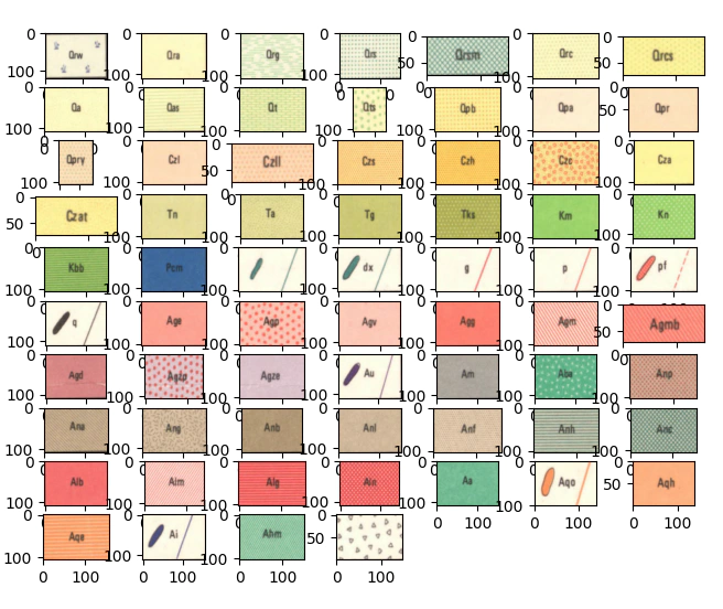
June 8, 2022 - 4 minutes read - 775 words

One of the failings of the previous model was that it didn’t encode texture, reviewing the stratigraphic units that we have in the map we can see that most of these units are encoded by both colour and texture.

Plot matrix of all the stratigraphic units

With this knowledge in hand we will try and create a model that uses a window rather than the single pixel that we’ve used in part 1.

If you’ve not downloaded the data used in the first article please start there, if you have then we can begin by loading the data and viewing the stratigraphic units.

from pathlib import Path 
import json
import imageio
import numpy as np
from matplotlib import pyplot as plt
# load the data that you've previously downloaded in part 1
outpath = Path('data')
outfile = outpath.joinpath('Collie_si5006_Geol_MGA.json')

with open(outfile,'r') as file:
    data = json.load(file)

scanned_map = outpath.joinpath('Collie_si5006_Geol_MGA.jp2')
img = imageio.imread(scanned_map)
# display the all of the stratigraphic codes
train_array = {}
for it,i in enumerate(data['shapes']):
    minx, miny = np.floor(i['points'][0]).astype(int)
    maxx, maxy =np.ceil(i['points'][1]).astype(int)
    ii,jj = np.ix_( range(miny,maxy),range(minx,maxx))
    aa = img[ii,jj,:]
    train_array.update({i['label']:aa})

for i,name in enumerate(train_array):
    if not name == 'TestSection':
        plt.subplot(7, 10,i+1)
        plt.imshow(train_array[name])
plt.show()

Let’s begin by extracting a set of training data to create the model, however this time we will be extracting a set of windows of for example 5x5 or 3x3 and then reshaping them into a 2d array that we can feed into CatBoost

# create the training datasets
from sklearn.feature_extraction.image import extract_patches_2d
from sklearn.model_selection import train_test_split
from catboost import CatBoostClassifier
from sklearn import metrics

x_tmp = []
y_tmp = []
colors = []

window = 11
n_sample = 300
iters = 0
for i in train_array:
    if not i == 'TestSection':
        tmp = train_array[i]
        tmp_win = extract_patches_2d(tmp,(window,window),max_patches=n_sample)
        # extract the colormap 
        tc = np.mean(tmp.reshape(-1,3),0)/255
        colors.append(tc)
        tmp_win = tmp_win.reshape(n_sample,window*window*3)
        tmp_labels = np.repeat(iters,n_sample).reshape(-1,1)
        x_tmp.append(tmp_win)
        y_tmp.append(tmp_labels)
        iters+=1

y = np.concatenate(y_tmp)
x = np.concatenate(x_tmp)

# generate train test and validation splits
split_size = y.shape[0]//3
xtraintest, xval, ytraintest, yval = train_test_split(x,y,test_size=split_size)
xtrain, xtest, ytrain, ytest = train_test_split(xtraintest,ytraintest,test_size=split_size)
# train our catboost model this time we are going to use the testing dataset that we've created to stop the model from overfitting. 
cbc = CatBoostClassifier(2000,od_type='IncToDec',od_pval=0.01, use_best_model=True)
cbc.fit(xtrain, ytrain, eval_set=(xtest, ytest))

After about 4 minutes of training we can then test the model’s performance, as we did in the last part we will have a sanity check of the model performance, this time however we will look at the validation data so that we have a better idea of the performance of the model on unseen data.

from sklearn import metrics
from matplotlib.colors import ListedColormap
# run the trained model and apply it to the validation data.
yhat = cbc.predict(xval)
# create the confusion matrix
cm = metrics.confusion_matrix(yval, yhat)
# taking the log of the confusion matrix is an easy way to set 0 values to white.
plt.imshow(np.log(cm))
plt.show()

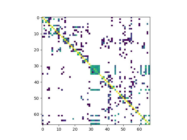
As we did last time we are going to look at the confusion matrix, ideally we would see only values down the diagonal of the image, but there are still significant numbers of misclassified items indicated by the coloured squares sitting off diagonal.

Leaving the performance of the classifier as it is we are going to apply it to our test section, so that we can visually check the performance and decide if this method is going to be at all prospective for futher investigation.

from scipy.signal import medfilt2d
from skimage.segmentation import mark_boundaries 

# application of model to test section
test_section = train_array['TestSection']
# get the size of the image
r,c,_= test_section.shape

# take sliding windows across the entire test section
test_window = extract_patches_2d(test_section,(window,window))
# reshape these windows into a 2d array
test_window = test_window.reshape(-1,window*window*3)
# run the model
win_hat = cbc.predict(test_window)
# calculation to get the shape of the output
rnew, cnew = (r-(window-1)),(c-(window-1))
# poff is the number of pixels lost when we create the sliding windows
poff = int((window-1)/2)
# create the color map so the image looks nice
cmap = ListedColormap(colors)
im_predict = win_hat.reshape(rnew,cnew)

# filter the model to smooth out the speckle 
im_filt = medfilt2d(im_predict,11)
# the resultant image is a little smaller than the image in the test section
# so we are removing a few pixels from the top and bottom
ts = test_section[poff:-poff,poff:-poff,:]
plt.imshow(mark_boundaries(ts,im_filt,color=[0,0,0]))
plt.show()

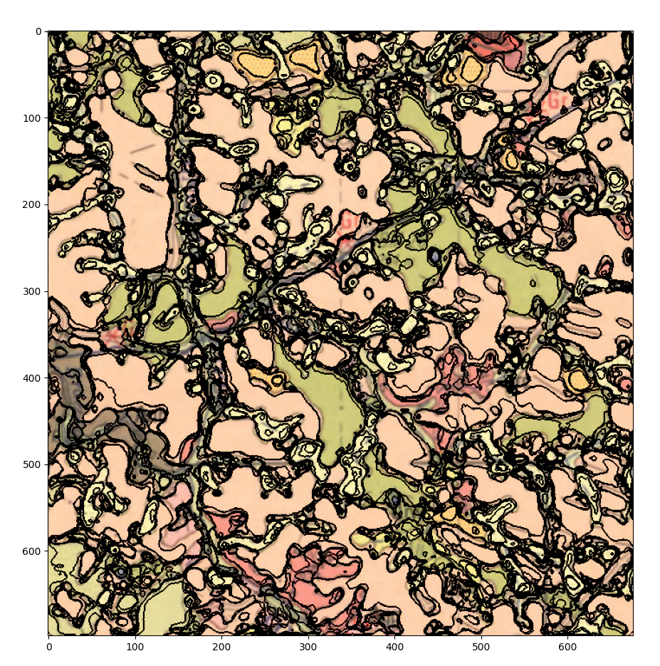
Let’s see what the performance looks like:

application of trained model applied to test section

I would say that it’s ok at a stretch there are far too many boundaries and not all the units are properly segmented, additionally the text and line work is still causing issues.

At this point we can probably give up on the path that we are on and move onto convolutional neural network models, but that can wait until the next episode.

Thanks,

Ben.