Contents

0. Intro
1. Configure Python
2. Simulation
3. Feature Extraction
4. References

Intro

I have become sick of copy and pasting feature extraction code around so I’ve updated pytsg to include some basic feature extraction methods.

To learn this new interface let’s discuss some common feature extraction methods for hyperspectral data, we are not going to touch on dimensionality reduction techniques like PCA as the interpretation is less obvious than scalar extraction techniques such as band ratios, polynomial fitting and gaussian decomposition. Also we won’t touch on more signal processing based methods such matched filters, wavelets or FFT because that is beyond basic feature extraction.

Configure Python

We need to begin this process by first installing the required libraries.

pip install matplotlib numpy pytsg

Simulation

Before we process real spectra let us first simulate simple spectrum so we that we can better understand the pros and cons of each method.

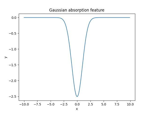
Let’s first start by simulating the simplest case, a single gaussian absorbtion representing a continuum removed feature.

import numpy as np
from matplotlib import pyplot as plt
from scipy.optimize import least_squares
from pytsg import feature

xrange = np.arange(0, 20, 0.1)
spectra = feature.gaussian(xrange, -1, 10, 1)
plt.plot(xrange, spectra.T)
plt.xlabel("x")
plt.ylabel("y")
plt.title("Gaussian absorption feature")
plt.show()

Feature Extraction

To understand some of the parameter interactions we will now apply the simple feature extractors to the simulated absorbtion feature.

wavelength = xrange
start, end = 8, 12
sqm_fit = sqm(xrange, spectra, 9, 11)
band_parameters = band_extractor(np.vstack([spectra] * 2))
# convert channel number to wavelength
band_parameters[:, 0] = xrange[band_parameters[:, 0].astype(int)]

gaussian_fit = fit_gaussian(xrange, spectra, x0=[1, 8, 5])
plt.plot(xrange, spectra.T, label="spectra")
plt.plot(
    band_parameters[0, 0],
    band_parameters[0, 1],
    "ko",
    label="band minimum and position",
)
plt.plot(xrange, poly.polyval(xrange, sqm_fit[0].T).T, label="sqm evaluated")
plt.plot(sqm_fit[1], sqm_fit[2], "r+", label="sqm band centre and depth")
plt.plot(
    [sqm_fit[3][0] / 2 + sqm_fit[1][0], sqm_fit[1][0] - sqm_fit[3][0] / 2],
    [0, 0],
    label="sqm feature width",
)

plt.ylim([-3, 1])
plt.legend()
plt.xlabel("wavelength")
plt.ylabel("Y")
plt.show()

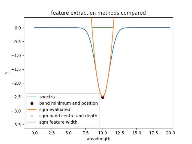
For the simple feature here we can see that both sqm and the band statistics provide practically the same feature depth and position.

It is important to note that band statistics only return feature position and depth while the sqm method estimates position, depth and width.

One of the more subtle aspects of processing is the behavior of these feature extraction algorithms for less than optimal conditions.

Firstly let’s assess how well we perform when modifying the position and band width of the absorbtion feature.

# vary the centre locations
centres = np.arange(-10, 10, 0.1)
channels = np.arange(-50, 50)
spectra = np.zeros((centres.size, channels.size))

for n, i in enumerate(centres):
    tmp = feature.gaussian(channels, -1,i, 1)
    spectra[n] = tmp


band_parameters = feature.band_extractor(spectra)

band_parameters[:, 0] = channels[band_parameters[:, 0].astype(int)]

feat, coef = feature.sqm(channels, spectra)

plt.plot(centres, centres - feat[:,0], label="sqm centre")
plt.plot(centres, centres - band_parameters[:, 0], ".", label="band minimum")
plt.xlabel("feature centre")
plt.ylabel("error")
plt.legend()
plt.show()

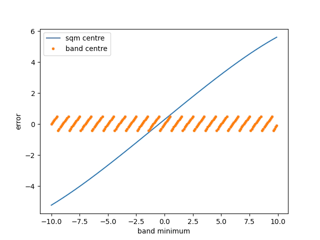
The plot below demonstrates an important point in that using the band statistics has a relatively constant error rate of at worst 1/2 of the channel resolution for a noiseless signal.

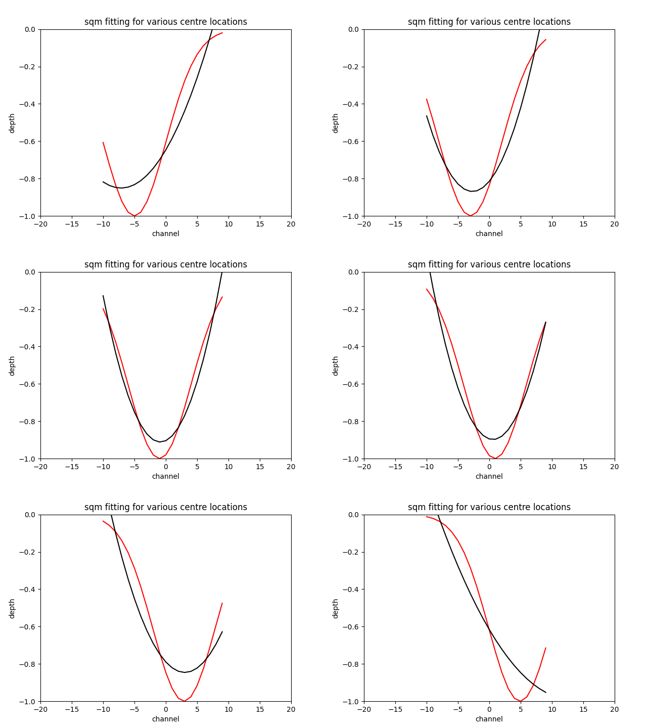
The sqm fit can acheive an excellent error if you are very close to the centre of the feature and the feature is centred on the window the gif below to demonstrates the effect.

N.B. Fitting a gaussian returns the original feature with around a tolerance of the optimiser, as long as you initialise the the optimiser around the correct location.

Bonus plotting for the gif:

from matplotlib.animation import FuncAnimation

# vary the centre locations
centres = np.arange(-5, 5, 0.1)
channels = np.arange(-10, 10)

fig, ax = plt.subplots()
xdata, ydata = [], []
(ln,) = ax.plot([], [], "r")
(f1,) = ax.plot([], [], "k")


def init():
    ax.set_xlim(-20, 20)
    ax.set_ylim(-1, 0)
    return (ln,)


def update(frame):
    tmp = feature.gaussian(channels, -1, frame, 5)
    stat, coef = feature.sqm(channels, tmp.reshape(1, -1))
    val = poly.polyval(channels, coef[0])

    ln.set_data(channels, tmp)
    f1.set_data(channels, val)

    return ln, f1


ax.set_title("sqm fitting for various centre locations")
ax.set_xlabel("channel")
ax.set_ylabel("depth")


ani = FuncAnimation(fig, update, frames=centres, init_func=init, blit=True, interval=10)
plt.show()

References

Laukamp, C.; Rodger, A.; LeGras, M.; Lampinen, H.; Lau, I.C.; Pejcic, B.; Stromberg, J.; Francis, N.; Ramanaidou, E. Mineral Physicochemistry Underlying Feature-Based Extraction of Mineral Abundance and Composition from Shortwave, Mid and Thermal Infrared Reflectance Spectra. Minerals 2021, 11, 347. https://doi.org/10.3390/min11040347

John M. Meyer, Raymond F. Kokaly, Elizabeth Holley, Hyperspectral remote sensing of white mica: A review of imaging and point-based spectrometer studies for mineral resources, with spectrometer design considerations, Remote Sensing of Environment, Volume 275, 2022, 113000, ISSN 0034-4257, https://doi.org/10.1016/j.rse.2022.113000.https://

Andrew Rodger, Carsten Laukamp, Maarten Haest, Thomas Cudahy, A simple quadratic method of absorption feature wavelength estimation in continuum removed spectra, Remote Sensing of Environment, Volume 118, 2012, Pages 273-283, ISSN 0034-4257, https://doi.org/10.1016/j.rse.2011.11.025. (https://www.sciencedirect.com/science/article/pii/S0034425711004226)