qaqc of field asd data
- 10 minutes read - 2106 wordsContents
Intro
Let’s run though an example of how to validate unseen spectral data. I was originally going to write about feature extraction but that can be for the next installment.
Often you get a data set of which you’ve had no association in collecting or know nothing about. So to demonstrate this workflow, I’m going to run through some spectral data that I’ve never seen before and a commodity that I’ve no experience with either. I had a search through the WAMEX database for some spectral data and found Paladin’s Carley bore deposit. I would like to thank Paladin for actually reporting the raw spectral files, rather than just the report or the interpreted results.
For this example we are going to use the data from the Paladin’s 2016 and 2015 carley bore annual report and also Energia Minerals 2012 carley bore report a roll front uranium deposit. Now I know nothing about roll front uranium but I’m not going to let being uncompetent stop me.
Configure Python
Let’s first install the required libraries.
pip install git+https://github.com/FractalGeoAnalytics/AuGeoscienceDataSets.git
pip install git+https://github.com/adamchlus/specIO.git
pip install matplotlib pandas numpy dhcomp pysptools
Get Data
Once the required libraries are installed let’s download the data and unpack the archives, we are pulling data from several annual reports so that we can have all the data that we require for the analysis as the assays, asd and the field data were collected at different times.
import specIO
from matplotlib import pyplot as plt
from pathlib import Path
import shutil
import numpy as np
from augeosciencedatasets import downloaders
import pandas as pd
from matplotlib import pyplot as plt

outpath = Path("data/ASDCarleyBore")
dasc_urls = {
    "A110793": (
        "Spectra.zip",
        "https://geodocsget.dmirs.wa.gov.au/api/GeoDocsGet?filekey=0586c4d5-1652-48fe-ad0a-a9fec71d7446-834jllo21jrjnkvgrbyqgce5w0sgr16gfot5nfps",
    ),
    "A97345": (
        "Drill.zip",
        "https://geodocsget.dmirs.wa.gov.au/api/GeoDocsGet?filekey=45ba37d4-0c14-440f-b68d-55c273c81721-7q7t19fnlrjaams5rtjl2cifylfkvicgcc9u4w5s",
    ),
    "A108383": (
        "Drill.zip",
        "https://geodocsget.dmirs.wa.gov.au/api/GeoDocsGet?filekey=375b639f-bdfe-402d-bdcc-6792f25588dc-vu7pjtg9j3ym9b4gb16rvcqtrsge9p1ilhxk4dtp",
    ),
}

if not outpath.exists():
    outpath.mkdir(parents=True)

for file in dasc_urls:
    outfile = outpath.joinpath(file, dasc_urls[file][0])
    if not outfile.parent.exists():
        outfile.parent.mkdir(parents=True)
    downloaders.from_dasc(dasc_urls[file][1], outfile)
    # unzip the zip file
    shutil.unpack_archive(outfile, outfile.parent)
Load the spectra
With our data extracted we will now run some rudimentary meta data extraction and jump correction between the detectors.
The ASD jump correction is better done by this method Cause, Effect, and Correction of Field Spectroradiometer Interchannel Radiometric Steps but I’m too lazy to do that for now.
For the moment I have just implement a very simple correction that removes the steps between detectors.
# here is my very lazy jump correction code
def bad_jump_corrector(spec):
    # get the splice positions
    pos_splice1 = np.argmin(np.abs(spec.refl.index - spec.splice1))
    pos_splice2 = np.argmin(np.abs(spec.refl.index - spec.splice2))
    # do a copy other wise we will work on the original array
    jump_corrected = spec.refl.values.copy()
    # get the first offset from the splice channel and the next
    off1 = jump_corrected[pos_splice1] - jump_corrected[pos_splice1 + 1]
    # get the second offset from the splice channel and the next
    off2 = jump_corrected[pos_splice2] - jump_corrected[pos_splice2 + 1]
    # add offset 1 to the second detector
    jump_corrected[pos_splice1 + 1 : (pos_splice2 + 1)] += off1
    # add both offset 1 and 2 to the 3rd detector positions
    jump_corrected[pos_splice2 + 1 :] += off2 + off1
    return jump_corrected


# list the spectra
spectra_names = ["refl", "refr", "targ"]
spectra_folder = outpath.joinpath("Spectra")
tmp_meta = []
tmp_spectra = []

# loop over each file and extract the meta data and the reflectance
# spectrum do a bad jump correction as well so it looks nice.
for file in spectra_folder.glob("*.asd"):
    spec = specIO.openASD(str(file))
    spectra_meta_names = [
        name
        for name in dir(spec)
        if (not name.startswith("__")) and not (name in spectra_names)
    ]
    # make a dataframe with the metadata
    tmp = {}
    for s in spectra_meta_names:
        value = getattr(spec, s)
        tmp.update({s: value})

    jc = bad_jump_corrector(spec)
    tmp_meta.append(tmp)
    tmp_spectra.append(jc)

# let's check out the quality of the bad jump corrector
plt.plot(spec.refl.index,jc,label='jump corrected')
plt.plot(spec.refl,label='raw')
plt.ylabel('reflectance')
plt.xlabel('wavelength')
plt.title('ASD Bad Jump Correction')
plt.legend()
plt.show()

# create a df of the spectra
wavelengths = spec.refl.index.values
spectra_columns = [f'w{s}'for s in spec.refl.index.astype(int)]
specdf = pd.DataFrame(np.stack(tmp_spectra), columns=spectra_columns)

# create a df of the meta
metadf = pd.DataFrame(tmp_meta)
# concatenate into a nice df of both
spectrum = pd.concat([metadf, specdf], axis=1)

# if you want save change save to True
SAVE = False
if SAVE:
    spectrum.to_csv(outpath.joinpath("Spectra.csv"))
Let’s check out the bad jump corrector:
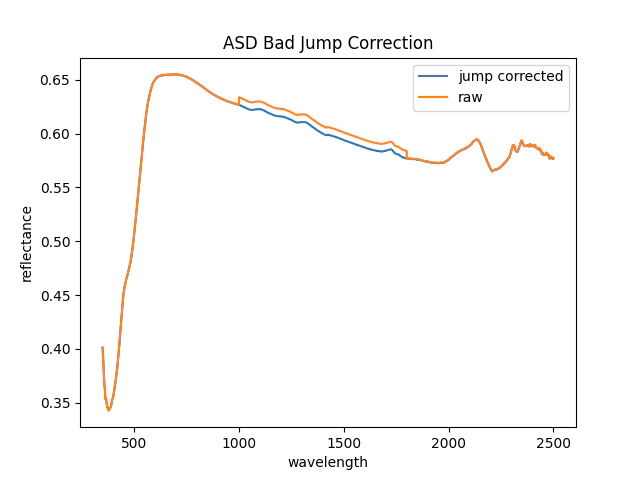
Thats good enough for me let’s continue.
Merging the assay and logging data
With our spectrum loaded now we need map the spectra to it’s interval because unfortunately the file names don’t contain the information that we need to map to the drill hole interval.
We load the processed aisiris csv and use that to map to the correct interval.
To assess the utility of the spectral data we load the stratigraphy, color,assay, grain size and alteration information from a few other annual reports.
# we also need to open the aiSiris results to get the
# mapping for the sample id and the hole, from and to information
aisirus = pd.read_csv(spectra_folder.joinpath("CB_aiSIRIS results.csv"))

from augeosciencedatasets import readers

tmp_assay = []
tmp_lith = []
tmp_scint = []
tmp_collar = []
tmp_xrf = []
# the column map is to correct some inconsistencies with the column names
column_map = {
    "mFrom": "DEPTH_FROM",
    "mTo": "DEPTH_TO",
    "SITE ID": "Hole_id",
    "SCINTILLOMETER": "CPS_AVERAGE",
}
# this maps the geo logged colours to the codes
# taken from 'data/ASDCarleyBore/A97345/App2_Energia_LibraryCodes_201302.pdf'

colors = {'B':'blue', 'E':'grey', 'G': 'green','H':'khaki','K':'pink','N':'black','O':'orange','P':'purple','R':'red','U':'umber','W':'white','Y':'yellow'}
intensity = {'D':'dark','L':'light','M':'medium'}

tmp_geo = {}
# loop over the each file and search for the .txt extension.
# look in the file name to see where to allocate the data
for i in outpath.glob("**/*.txt"):
    tmp, tmp_head = readers.dmp(i)
    if i.name.find("ASS") >= 0:
        tmp_assay.append(tmp)
    elif i.name.find("LITH") >= 0:
        tmp_lith.append(tmp)
    elif i.name.find("SCINT") >= 0:
        tmp.rename(columns=column_map, inplace=True)
        tmp_scint.append(tmp)
    elif (i.name.find("COLL") >= 0) and (i.parts[2] == "A108383"):
        tmp_collar.append(tmp)
    elif i.name.find("XRF") >= 0:
        tmp.columns = [n.replace("_HHXppm", "") for n in tmp.columns.to_list()]
        tmp.rename(columns=column_map, inplace=True)
        tmp_xrf.append(tmp)
    elif (i.name.find("GEO") >= 0) or (i.name.find("ALT") >= 0):
        tmp_geo.update({i.stem:tmp})
    else:
        pass

# concatenate the data
assay = pd.concat(tmp_assay)
lith = pd.concat(tmp_lith)
scint = pd.concat(tmp_scint)
collar = pd.concat(tmp_collar)
pxrf = pd.concat(tmp_xrf)
# deal with the geological data types
strat = tmp_geo['CB_WADL4_GEO2015A']# stratigraphy
color = tmp_geo['CB_WADL4_GEO2015A_1']# colour
grain = tmp_geo['CB_WADL4_GEO2015A_2']# grain size
alter = tmp_geo['CB_WADL4_ALTE2015A']# alteration

# merge the assay to the aisiris data
assay_aisiris = pd.merge(
    assay,
    aisirus[["HoleId", "SampleId", "Spectrum"]],
    left_on=["HOLEID", "SAMPLE_ID"],
    right_on=["HoleId", "SampleId"],
)

# merge the spectra  to the assay and aisiris data
assay_spectrum = assay_aisiris.merge(spectrum,left_on='Spectrum', right_on='filename')
Validate the merge
We now have a mapping between the spectrum file name and the assays which we can use to validate the data collection process. For this check we are most interested in is confirming that the spectra and the assays are correctly joined.
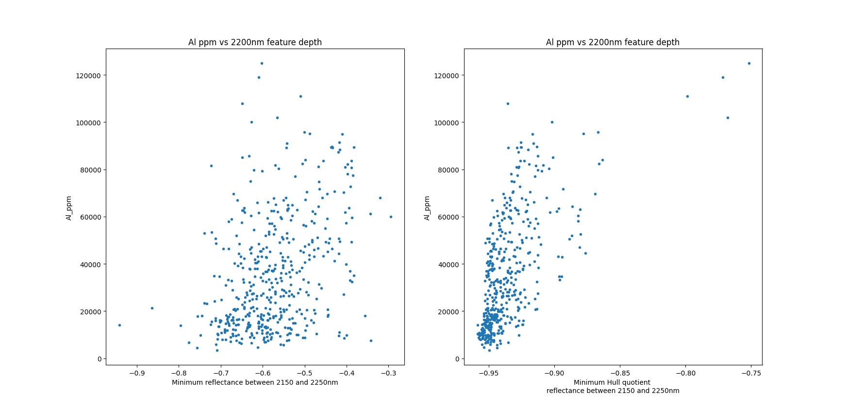
Using the relationship between the 2200nm feature and the Al concentration we can validate the merge.
If the data collection and the merge were good we should see a nice relationship between those two parameters.
We use the hull quotient spectra as we want to remove the variation in the reflectance, for comparison we can use the raw spectra with out the hull removal which has a significantly worse correlation, making it more difficult to decide if we are fooling ourselves.
# quick sanity check plot the Al against the total area of the 2200mn feature
# just to make sure that have correctly joined the data
ss = assay_spectrum[spectra_columns].values
ispec = (spec.refl.index>2150) & (spec.refl.index<2250)

import pysptools.spectro as spectro
hull_removed = np.zeros_like(ss)
for i,s in enumerate(ss):
    fea = spectro.SpectrumConvexHullQuotient(s.tolist(), wavelengths.tolist())
    hull_removed[i,:]=np.asarray(fea.get_continuum_removed_spectrum())


plt.subplot(1, 2, 1)
plt.plot(-np.min(ss[:,ispec],1),assay_spectrum.Al_ppm.astype(float),'.')
plt.xlabel('Minimum reflectance between 2150 and 2250nm')
plt.ylabel('Al_ppm')
plt.title('Al ppm vs 2200nm feature depth')

plt.subplot(1, 2, 2)
plt.plot(-np.min(hull_removed[:,ispec],1),assay_spectrum.Al_ppm.astype(float),'.')
plt.xlabel('Minimum Hull quotient \nreflectance between 2150 and 2250nm')
plt.ylabel('Al_ppm')
plt.title('Al ppm vs 2200nm feature depth')
plt.show()
Merge geological data
Now we have a level of confidence in the merge between assays and the rest of the data, let’s now merge the stratigraphy, colour, grainsize and alteration data.
The geological data is across multiple intervals so we will use dhcomp to merge the intervals.
# merge the geodata
from dhcomp import composite
def nan_clean(x):
    if x == None:
        y = 0
    elif isinstance(x, str) and (len(x)>0):
        y = float(x)
    elif x == '':
        y = 0
    else:
        y = 0
    return y

def composite_merge(primary, secondary,primary_bhid, primary_from, primary_to, secondary_bhid, secondary_from, secondary_to, secondary_columns):
    # loop over each bhid that is in both tables
    primary = primary.copy()
    pbhid = primary[primary_bhid].unique()
    sbhid = secondary[secondary_bhid].unique()
    bhids = set(pbhid).intersection(sbhid)
    # create space for the data
    primary[secondary_columns] = 0
    for bhid in bhids:
        idxbhidprimary = primary[primary_bhid] == bhid
        idxbhidsecondary = secondary[secondary_bhid] == bhid
        tmp_p = primary[idxbhidprimary]
        tmp_s = secondary[idxbhidsecondary]
        result,_ = composite.composite(tmp_p[primary_from].astype(float).values,tmp_p[primary_to].astype(float).values, tmp_s[secondary_from].astype(float).values, tmp_s[secondary_to].astype(float).values,tmp_s[secondary_columns].astype(float).values)
        primary.loc[idxbhidprimary, secondary_columns] = result
    return primary


def get_color(x):
    if isinstance(x, str) and (len(x)>0):
        if x[0] in intensity:
            y = colors[x[1].upper()]
        else:
            y = colors[x[0].upper()]
    else:
        y =''
    return y

lith['MAJCOLOR'] = lith.COLOUR1.map(get_color)
lith['Depth From'] = lith['DEPTH_FROM']
lith['Depth To'] = lith['DEPTH_TO']
lith['Hole_id'] = lith['HOLEID']

primary_bhid = 'HOLEID'
primary_from = 'DEPTH_FROM'
primary_to = 'DEPTH_TO'
# convert objects to float
assay_spectrum[primary_from] = assay_spectrum[primary_from].astype(float)
assay_spectrum[primary_to] = assay_spectrum[primary_to].astype(float)
secondary_bhid = 'Hole_id'
secondary_from = 'Depth From'
secondary_to = 'Depth To'
target_columns = [['STRATIGRAPHY'], ['MAJCOLOR'],['SHALE SIZE FACIES','FINESAND SIZED FACIES', 'COARSESAND SIZED FACIES'], ['Alteration']]
for secondary, columns in zip([strat,lith, grain, alter],target_columns):
    secondary[secondary_from] = secondary[secondary_from].astype(float)
    secondary[secondary_to] = secondary[secondary_to].astype(float)
    if len(columns) == 1:
        if columns[0] == 'Colour':
            secondary[columns[0]] = secondary[columns[0]].str.upper()
        dummies = pd.get_dummies(secondary[columns[0]])
        secondary = pd.concat([secondary, dummies],axis=1)
        secondary_columns  = dummies.columns
    else:
        for g in columns:
            secondary[g] = secondary[g].map(nan_clean)
        secondary_columns = columns
    assay_spectrum = composite_merge(assay_spectrum, secondary, primary_bhid, primary_from, primary_to, secondary_bhid, secondary_from, secondary_to, secondary_columns)
Logged Colour
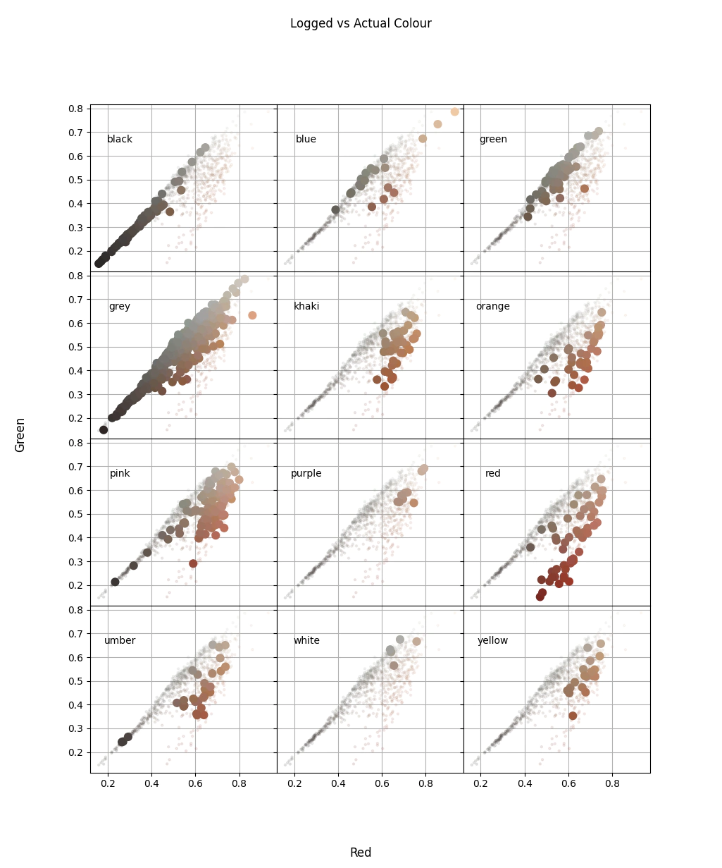
If you don’t have assays and would like to confirm that you’ve merged the data correctly we would be forced to look at the logging data. I suspect the simplest and most reliable parameter to log is colour, so let’s convert the regression problem into classification.
Before going to far with the classification let’s check how the colour labels plot in comparison to the hylogger measured colour.
# let's amuse outselves by cheking the geo colours
spec_col = assay_spectrum[['w625', 'w525','w460']].values

# recode the colour
majority_color = assay_spectrum.loc[:,assay_spectrum.columns.isin(colors.values())].idxmax(1)

minc = spec_col.min(0)
maxc = spec_col.max(0)

fig, ax = plt.subplots(4, 3,
                       sharex=True,
                       sharey=True)
plt.subplots_adjust(hspace=0,
                    wspace=0)
reverse_codes = {colors[c]:c for c in colors}
for n,i in enumerate(np.unique(majority_color)):
    idx = majority_color == i
    # send the grid to the back
    ax.ravel()[n].set_axisbelow(True)
    ax.ravel()[n].grid()
    ax.ravel()[n].scatter(spec_col[~idx,0], spec_col[~idx,1],s=5,color=spec_col[~idx],alpha=0.1)
    ax.ravel()[n].scatter(spec_col[idx,0], spec_col[idx,1],color=spec_col[idx],s=60)
    itxt ='{}\n{}'.format(i,reverse_codes[i])
    ax.ravel()[n].text(minc[0], maxc[1],i, horizontalalignment='center',verticalalignment='center', transform=ax.ravel()[n].transAxes)

plt.suptitle('Logged vs Actual Colour')
fig.supxlabel('Red')
fig.supylabel('Green')

plt.show()
Ideally we would have perfect separation between different the groups, unfortunately the image below shows some overlap between the colour groups but at least the data is not totally random.
We will now move to training a model to determine colour labels from the measured colours, for the sake of simplicity we are going to train a very basic model as we are trying to understand how the classes overlap. As with the relationship between Al and the 2200nm feature we expect that we can separate the classes, however as colour can be a notoriously difficult thing to agree on we must temper our expectations.
from sklearn.svm import SVC
from sklearn.metrics import confusion_matrix, ConfusionMatrixDisplay
from sklearn.metrics import balanced_accuracy_score

model = SVC().fit(spec_col,majority_color)

balanced_accuracy_score(majority_color, model.predict(spec_col))
cm = confusion_matrix(majority_color, model.predict(spec_col),normalize='pred')
disp = ConfusionMatrixDisplay(confusion_matrix=cm, display_labels=np.unique(majority_color))
disp.plot()
plt.show()
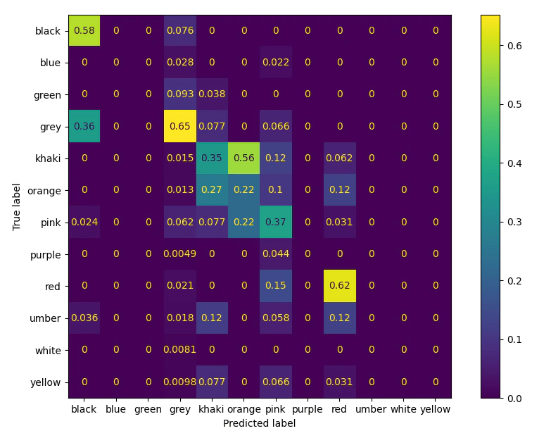
The performance is not great but it is not random, which indicates that there is some level of consistency in the colour logging, but it is very likely effected by typos or difficulty in remembering the codes.
From the confusion matrix we can see that there is a lot of mis-classification between the reddish colours, (pink, red, orange, khahki) and much less between black and grey (though the grey may be due to removing the intensity value i.e. dark grey)
To finish off and to make a short argument for simplifying the total number of codes that you have, we plot mean colours of the decision boundary of the classifier.
import matplotlib
from sklearn.inspection import DecisionBoundaryDisplay
from sklearn.svm import SVC
linx = np.linspace(spec_col[:, 0].min()*0.8, spec_col[:, 0].max()*1.2,200)
liny = np.linspace(spec_col[:, 1].min()*0.8, spec_col[:, 1].max()*1.2,200)
feature_1, feature_2 = np.meshgrid(linx,liny)

grid = np.vstack([feature_1.ravel(), feature_2.ravel()]).T

# fit a basic classifier
tree = SVC().fit(spec_col[:,0:2],pd.Categorical(majority_color).codes)

y_pred = np.reshape(tree.predict(grid), feature_1.shape)

display = DecisionBoundaryDisplay(xx0=feature_1, xx1=feature_2, response=y_pred)
# predict on the actual labels what the smoothed labels would be
labels = tree.predict(spec_col[:,0:2])

# create a colour map with the measured colours and colour the image by that
tmp_colours = pd.DataFrame({'labels':labels,'r':spec_col[:,0],'g':spec_col[:,1],'b':spec_col[:,2],}).groupby(['labels']).mean()
tmp_colours['color']= pd.Categorical(majority_color).categories[tmp_colours.index]

colmap = [i[1][['r','g','b']].values for i in tmp_colours.iterrows()]

cmap = matplotlib.colors.ListedColormap(colmap)
display.plot(cmap =cmap)
display.ax_.scatter(spec_col[:, 0], spec_col[:, 1], c=spec_col,edgecolors='black',s=60)
display.ax_.set_xlabel('Red')
display.ax_.set_ylabel('Green')
# plot the labels colours on the image with text
for i in tmp_colours.iterrows():
    plt.text(i[1].r,i[1].g,i[1].color,color='white')
plt.title('Decision Boundary for Logged vs Measured Colours')
plt.show()
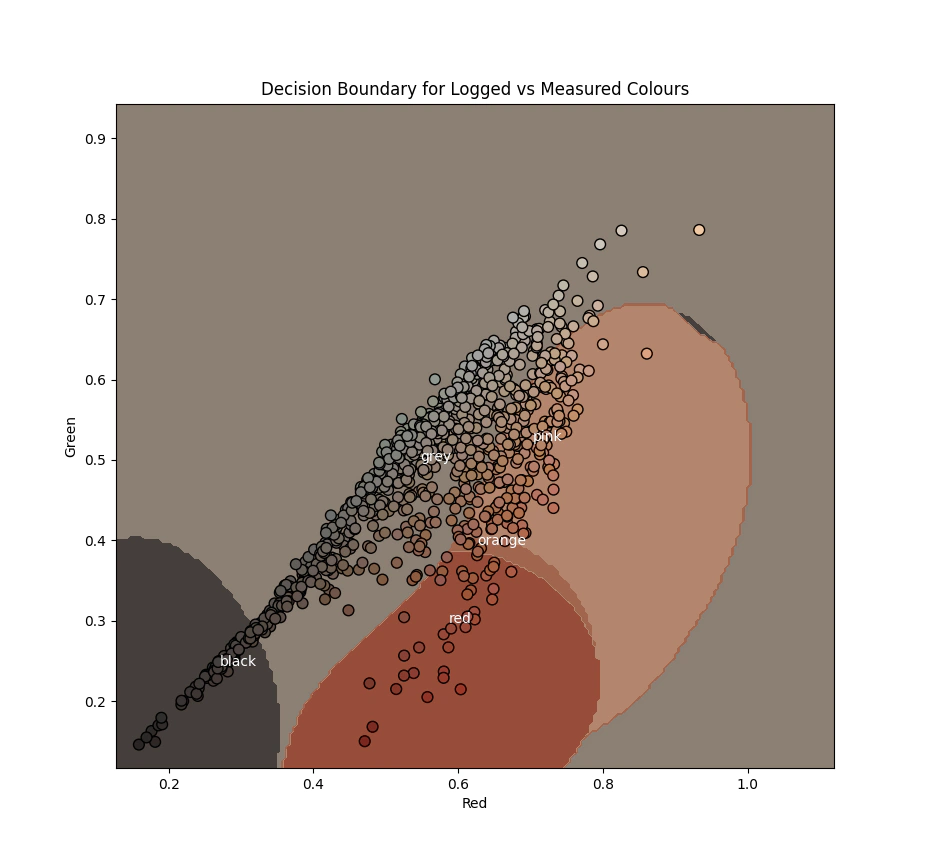
Thanks,
Ben.
References
Hueni, Andreas & Bialek, Aga. (2017). Cause, Effect, and Correction of Field Spectroradiometer Interchannel Radiometric Steps. IEEE Journal of Selected Topics in Applied Earth Observations and Remote Sensing. PP. 1-10. 10.1109/JSTARS.2016.2625043.