As an update to the last post on drill compositing, I’ve implemented a limited set of algorithms for the hard boundary compositing of drill hole intervals. It is important to note that the hard boundary aggregation algorithms must honor the smaller intervals in the drill hole.

All of the implementations I have seen utilise a version of what I have implemented as the greedy method.

One of the issues I have with the greedy algorithm is that there is no guarantee that the solution for a given drill hole is closest to the optimum i.e. the overall distance between target interval and the actual interval is minimised.

So to satisfy my desire for a solution I have implemented a novel or at to my knowledge never published, algorithm for finding the optimal set of composites that honor sample boundaries.

I use Dijkstra’s algorithm to find an optimal path through a set of depth intervals that are as close as possible to the desired interval length. Because it is important to cherry pick examples that demonstrate the superiority of your method here is one degenerate case showing where the greedy algorithm breaks down.

First we need to install the packages.

pip install dhcomp matplotlib

We can now show how much better the global compositing method is with this example:

from dhcomp.composite import HardComposite, _greedy_composite,_global_composite

import numpy as np
from matplotlib import pyplot as plt

# Compute position of nodes

depths = np.asarray([0, 1.9, 3.9, 5, 5.8, 7.9, 8])

global_composites = _global_composite(depths,2)
greedy_composites = _greedy_composite(depths,2)
print(np.diff(global_composites))
print(np.diff(greedy_composites))

Here we see that the global compositing function returns the following composited lengths of [ 1.9, 2, 1.9, 2.2 ].

The greedy algorithm returns [3.9, 4, 0.1], the standard solution here is to add a minimum length constraint to the algorithm and append any short intervals to the one that preceeds it.

global_composites = _global_composite(depths,2,min_length=1)
greedy_composites = _greedy_composite(depths,2,min_length=1)
global_composites_min_length = _global_composite(depths,2,min_length=1)
greedy_composites_min_length = _greedy_composite(depths,2,min_length=1)
print(np.diff(global_composites_min_length))
print(np.diff(greedy_composites_min_length))

With this setting we see no change to the global solution but the greedy algorithm has the last short interval appended to the middle interval and the greedy algorithm now returns [3.9, 4.1].

In this scenario the global solution is within 10% of the target interval length. While the greedy solution is 100% over the target length.

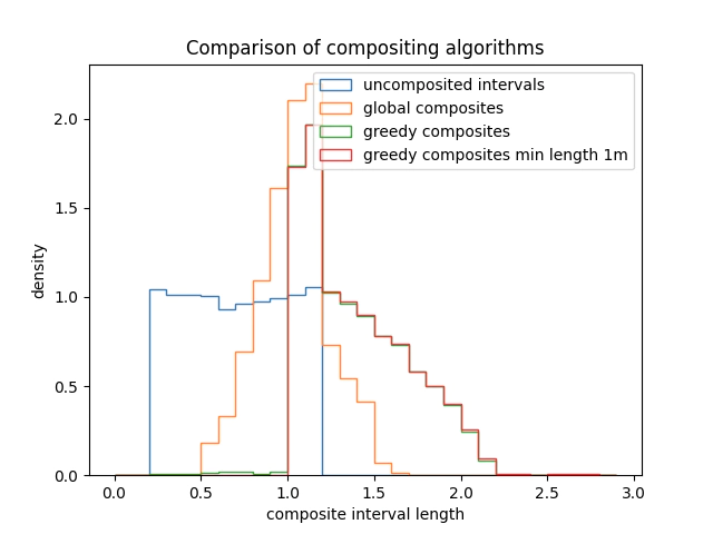
To preempt any complaints about cherry picking here is an example where we simulate the performance of each method using a random distribution of sample intervals.

interval = 1
global_depths = []
greedy_depths_constraint = []
greedy_depths = []
depths = []
for i in range(100):
    rlens = np.random.uniform(0.2, 1.2, 100)
    sfrom = np.concatenate([[0], np.cumsum(rlens).ravel()])
    sample_from, sample_to = sfrom[0:-1], sfrom[1:]

    array = np.ones_like(sample_from).reshape(-1, 1)
    depths.append(sample_to-sample_from)
    tmp_greedy, _, _ = HardComposite(
        sample_from, sample_to, array, interval=interval, method="greedy"
    )
    tmp_greedy_cons, _, _ = HardComposite(
        sample_from, sample_to, array, interval=interval, method="greedy", min_length=1
    )

    tmp_global, _, _ = HardComposite(
        sample_from, sample_to, array, interval=interval, method="global"
    )
    global_depths.append(tmp_global)
    greedy_depths.append(tmp_greedy)
    greedy_depths_constraint.append(tmp_greedy_cons)

gd = np.vstack(greedy_depths)
ad = np.concatenate(depths)
gdc = np.vstack(greedy_depths_constraint)

gld = np.vstack(global_depths)
mv = np.round(max(np.diff(gld).max(), np.diff(gd).max(),np.diff(gdc).max()))

plt.hist(ad, np.arange(0, mv, 0.1), histtype="step", density=True,label='uncomposited intervals')
plt.hist(np.diff(gld), np.arange(0, mv, 0.1), histtype="step", density=True,label='global composites')
plt.hist(np.diff(gd), np.arange(0, mv, 0.1), histtype="step", density=True,label='greedy composites')
plt.hist(np.diff(gdc), np.arange(0, mv, 0.1), histtype="step", density=True,label='greedy composites min length 1m')

plt.xlabel('composite interval length')
plt.ylabel('density')
plt.legend()
plt.title('Comparison of compositing algorithms')
plt.show()

Inspecting the image below we can see that the global method returns a pretty well centred and unbiased distribution centred around the target interval.

The greedy algorithm has more samples above the target interval length and a few intervals that are shorter than the target length. As discussed earlier including the minimum length constraint fixes this issue but there are many more samples that are much longer than the targeted sample length.

Finally it’s worth noting that while the global compositing algorithm is generally better performing with respect to matching the target interval for random intervals.

When you have regular samples lengths it’s generally better to use the greedy algorithm as it is faster and predictable. In particular you will always have the longer or shorter interval at either the start or end of the drill hole depending on algorithm direction.

Also as I haven’t needed to manage gaps (core loss) or internal dilution so they are not implemented. Therefore any intervals that contain nan values will return a nan.

Thanks,

Ben

References

J Davis, (2014), Website http://www.johndavis.co.uk/Portfolio/geobasys/compositing.htm

A.M Vargas, pygslib, (2018), GitHub repository, https://github.com/opengeostat/pygslib

J Hoffimann,(2018),GitHub repository, https://github.com/JuliaEarth/DrillHoles.jl