colour from hyperspectral

September 9, 2023 - 4 minutes read - 843 words

Good Morning All,

I’ve been wondering if the method I’ve been using to convert the hyperspectral colour to RGB was accurate and looked into the conversion of spectra to RGB values a bit further.

So to compare the accuracy of our spectra to rgb conversion code I’m going to use the data from the A98437 the 2013 Manyingee Uranium Annual report

We will compare the mean colour of the chips from the images to the rgb channel responses as used in the previous post and the correct method using the colour matching functions.

Because I am a helpful sort let’s work through this example with python so that you can calculate your own colours.

We need to configure our python install

pip install pytsg matplotlib colour-science
pip install git+https://github.com/FractalGeoAnalytics/AuGeoscienceDataSets.git

And download and unpack the required data

from pytsg import parse_tsg
from pathlib import Path
import numpy as np
from matplotlib import pyplot as plt
from colour import MSDS_CMFS
import colour
from augeosciencedatasets import downloaders
import shutil

from matplotlib import pyplot as plt
from matplotlib.patches import Rectangle
outpath = Path("data/A98437")

dasc_urls = {
    "": (
        "Spectral.zip",
        "https://geodocsget.dmirs.wa.gov.au/api/GeoDocsGet?filekey=9232823f-d099-4b28-beb1-4884b26f37b9-ebnsw3vxhn11utos9lm41y5vttty06jpydxc5szi",
    ),
}

if not outpath.exists():
    outpath.mkdir(parents=True)

for file in dasc_urls:
    outfile = outpath.joinpath(file, dasc_urls[file][0])
    if not outfile.parent.exists():
        outfile.parent.mkdir(parents=True)
    downloaders.from_dasc(dasc_urls[file][1], outfile)
    # unzip the zip file
    shutil.unpack_archive(outfile, outfile.parent)

path = Path("data/A98437/HyChips")
data = parse_tsg.read_package(path, read_cras_file=True)

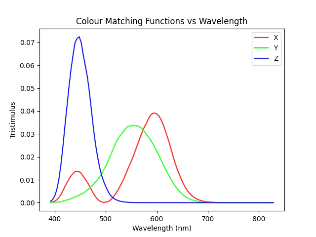
We will are going to use the CIE 2015 10 Degree Standard Observer, plotting these functions for each of the wavelengths in the hylogger data between 390 and 830nm we can see that there significant overlap between each of the colour matching functions.

Unlike the previous work where we simply selected 3 bands at approximately the far boundaries of the CIE Colour space.

# apparently this is the recommended observer
cmfs = MSDS_CMFS["CIE 2015 10 Degree Standard Observer"]

idxwave = (data.nir.wavelength <= 830) & (data.nir.wavelength >= 390)

tristim = colour.wavelength_to_XYZ(data.nir.wavelength[idxwave], cmfs)
tristim = tristim / np.sum(tristim, axis=0)

spec_xyz = data.nir.spectra[:, idxwave] @ tristim
spec_xyY = colour.XYZ_to_xyY(spec_xyz)

plt.plot(data.nir.wavelength[idxwave], tristim[:, 0], color=[1, 0, 0], label="X")
plt.plot(data.nir.wavelength[idxwave], tristim[:, 1], color=[0, 1, 0], label="Y")
plt.plot(data.nir.wavelength[idxwave], tristim[:, 2], color=[0, 0, 1], label="Z")
plt.legend()
plt.title("Colour Matching Functions vs Wavelength")
plt.xlabel("Wavelength (nm)")
plt.ylabel("Tristimulus")
plt.show()

I’m going to validate my colour calculations from the spectra against the mean colour of the pulp from the images of the trays, I assume that this colour is pretty much correct and we will try to best match this.

Let’s plot the first section of the tray, here we can see that we need to remove the from the image the sticker sheet and some of the instrument itself.

As the hylogger data is very consistent we assume that we can use a fixed offset to calculate the mean colour for each section of the tray.

n_spectra = data.nir.spectra.shape[0]
tray_image_rows = data.cras.image.shape[0] // n_spectra
# calculate the mean rgb colour for the image array
# we use the fixed offset here as the trays are fixed
#  in place by the hychips system.
# also we need to divide by 255 to get the rgb values between 0 and 1
rgb = data.cras.image[:, 200:600, :].mean(1) / 255
# xyY colour space is my new favourite
image_xyY = colour.XYZ_to_xyY(colour.sRGB_to_XYZ(rgb))

# tile an index
sidx = np.repeat(np.arange(0, n_spectra), tray_image_rows)

rgb_mean = []
# loop over each position in the spectra and
# take the mean rgb of the image
for i in np.arange(n_spectra):
    ssidx = sidx == i
    trgb = rgb[ssidx][0:250].mean(0)
    rgb_mean.append(trgb)

# create a numpy array
rgb_mean = np.stack(rgb_mean)
# convert to xyY cause I like that
xyY_mean = colour.XYZ_to_xyY(colour.sRGB_to_XYZ(rgb_mean))

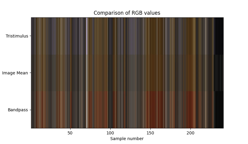
With the mean colour calculated for each image we can now compare the colour between the original band pass method, the RGB from the camera and the current colour matching function based method.


r, g, b = (
    np.argmin(np.abs(data.nir.wavelength - 625)),
    np.argmin(np.abs(data.nir.wavelength - 525)),
    np.argmin(np.abs(data.nir.wavelength - 460)),
)
rgb_bandpass = data.nir.spectra[:, [r, g, b]]
ax = plt.subplot()
for i in range(240):
    ax.add_artist(Rectangle((i + 1, 0), 1, 1, color=rgb_mean[i], fill=True))
    ax.add_artist(Rectangle((i + 1, 1), 1, 1, color=rgbspec[i], fill=True))
    ax.add_artist(Rectangle((i + 1, -1), 1, 1, color=rgb_bandpass[i], fill=True))

plt.yticks([0.5, 1.5, -0.5], ["Image Mean", "Tristimulus", "Bandpass"])
plt.ylim(-1, 2)
plt.xlim(1, 241)
plt.xlabel('Sample number')
plt.title("Comparison of RGB values")
plt.show()

Comparing the results between the band pass method and colour matching compared to the mean RGB colour from the image we can see that the band pass method is very red in comparision to the mean rgb from the camera, where as the colour matching function is very close to the image mean colour.

I’m tempted to conclude that the differences between the image mean colour and the spectral colour are due to minor differences in the transfer functions between methods.

And I also assume here that the spectral colours are correct.

Thanks,

Ben.

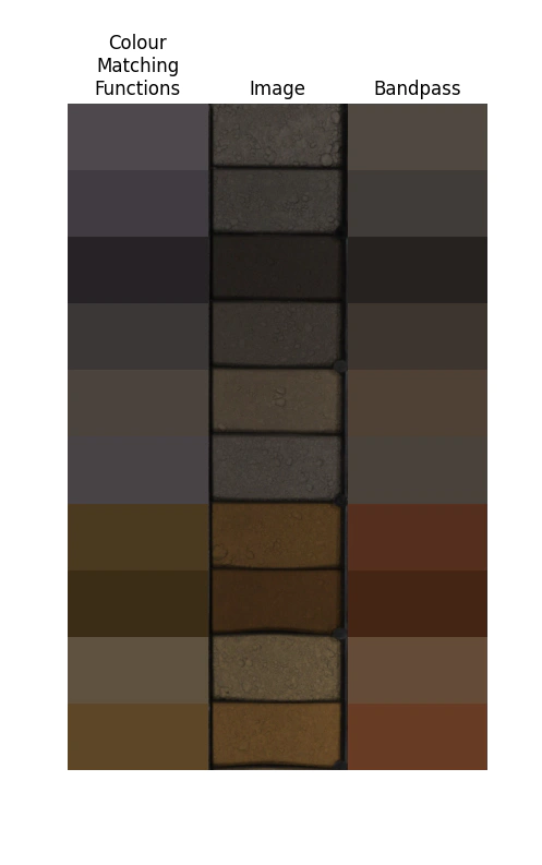
P.S bonus plot cause I thought it looked nice.

Comparison between colour matching functions bandpass and sRGB image mean


nplot = 20
fig, ax = plt.subplots(nplot, 3)
plt.subplots_adjust(hspace=0,
                    wspace=0)

for i in range(nplot):
    ax[i,0].add_patch(Rectangle((0, 0), 1, 1, color=rgbspec[i], fill=True))
    ax[i,1].imshow(data.cras.image[i * 279 : (i + 1) * 279, 69:653, :])
    ax[i,2].add_patch(Rectangle((0, 0), 1, 1, color=rgb_bandpass[i], fill=True))
    for j in range(3):
        ax[i,j].axis('off')
    if i == 0:
        ax[i,0].set_title("Colour\nMatching\nFunctions")
        ax[i,1].set_title("Image")
        ax[i,2].set_title("Bandpass")
plt.show()