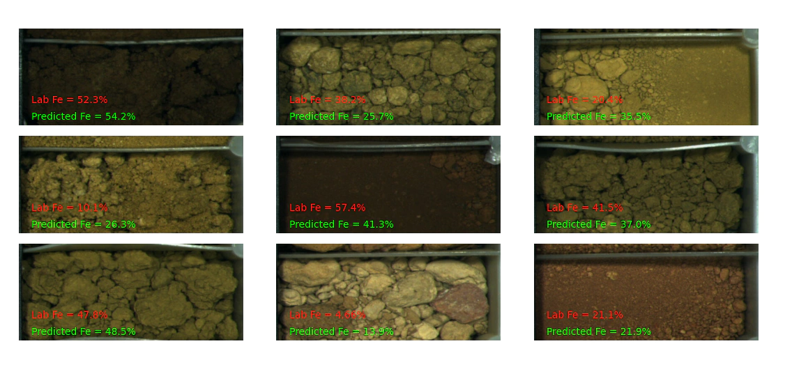
chip imagery and hyperspectral
- 6 minutes read - 1150 words
Let’s talk about the performance of using chips vs hyperspectral to classify ore and waste in an Iron ore deposit.

Before we go onto the technical work let’s discuss the practical uses of this information. Common use cases would be deciding if a sample is ore/waste, screening samples for further analysis or simply selecting the right sensor for you application and trading off cost/speed/performance/technical difficulty considerations.
So with all that in mind I hope that you will find a smart application in your workplace.
As we did last time we are going to use the data from the C3DMM project we will use the information from the cras.bip file as well and extract the imagery.
Also because we like fun, we are going to flow some tensors with tensorflow.
Let’s install the required libraries.
pip install pip install pytsg
pip install matplotlib numpy tensorflow tensorflow_hub
We need to download a dataset I stole this code from the last article and added the cras file for the imagery.
import json
import urllib.parse
import urllib.request
from pathlib import Path

# we are going to use the swagger api to get the files from here programatically this first call here is to list all the available files
url =  'https://data.csiro.au/dap/ws/v2/collections/44783v1/data'
with urllib.request.urlopen( url ) as response:
    response_text = response.read()
# the variable response_text is returned as a json package we are going to parse
# it with the python json library
c3dmm_files = json.loads(response_text)
base_dir = Path('data/')

# here is a list of the target files that we are going to need to
# do this experiment
target_files = ['RC_data.bip','RC_data.tsg','RC_data_cras.bip']

# loop over each of the files in the json
# if you've already downloaded them then we won't download the files again.
for i in c3dmm_files['file']:
    # pathlib makes path handling simple I prefer it generally over the os library
    fname = Path(i['filename'])
    url = i['link']['href']
    # if the file names is in the list of target files let's download
    if fname.name in target_files:
        outfile = base_dir.joinpath(fname)
        # check if the folder exists if not make it
        if not outfile.parents[0].exists():
            outfile.parent.mkdir(parents=True,exist_ok=True)
        # check if the file exists if it does then don't download
        if not outfile.exists():
            # download the file
            with urllib.request.urlopen( url ) as response:
                response = response.read()
                with open(outfile,'wb') as file:
                    file.write(response)
Before we can do any analysis we need to pre-process the images out of the cras file and into something that we can process.
The simplest way to achieve this is to use the newly developed functionality in pytsg and extract “depth registered” images from the software.
from pytsg.parse_tsg import read_tsg_bip_pair,extract_chips
inputfolder = base_dir.joinpath('drill hole data/RC_hyperspectral_geochem')
tsg_file = inputfolder.joinpath('RC_data.tsg')
bip_file = inputfolder.joinpath('RC_data.bip')
cras_file = inputfolder.joinpath('RC_data_cras.bip')
image_folder= inputfolder.joinpath('img')
# read the spectra
nir = read_tsg_bip_pair(tsg_file, bip_file,'nir')
# extract the images from the cras file
extract_chips(cras_file,image_folder,nir)
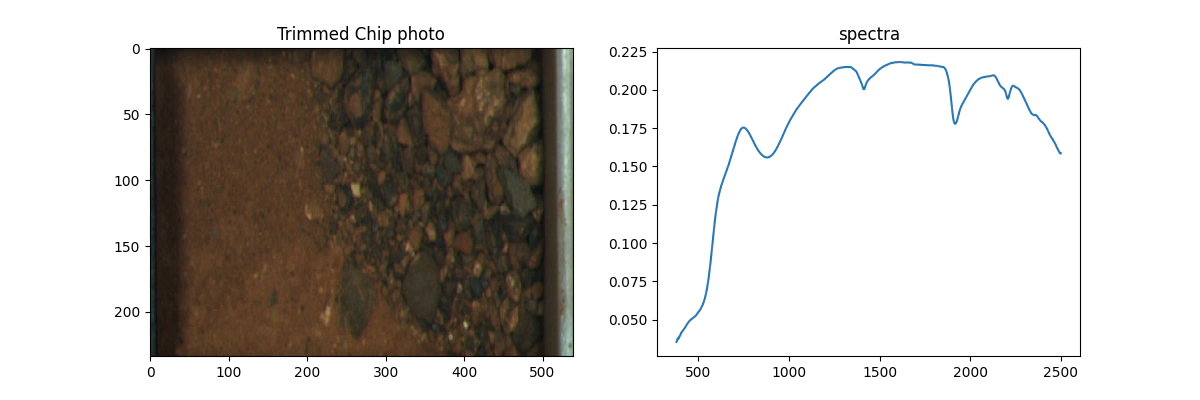
It is important to plot pictures for sanity checking purposes.

Follow the code section below to make your own.
# collate a list of the images
# and pair them to the scalars
from matplotlib import pyplot as plt
scalars = nir.scalars.copy()
scalars['jpg'] = ''
for i in Path(image_folder).glob('*.jpg'):
    idx_pair = scalars.Index.astype(int) == int(i.stem)
    scalars.loc[idx_pair,'jpg'] = i

# now we can look at paired spectra and images
import simplejpeg
jpg = scalars.loc[0].jpg
with open(jpg,'rb') as f:
    jbytes= f.read()
    img = simplejpeg.decode_jpeg(jbytes)

# make a nice picture because we like pictures
plt.figure(figsize=(12, 4))
plt.subplot(1, 2, 1)
plt.imshow(img[:,461:1000,:],aspect='auto')
plt.title('Trimmed Chip photo')
plt.subplot(1, 2,2)
plt.plot(nir.wavelength,nir.spectra[0])
plt.title('spectra')
plt.show()
Finally we can do some fun stuff. You could train a CNN from scratch but unless you have a lot of data and a lot of compute you are better off using pre-trained models and fine tuning. With that in mind let’s go to tfhub and get a nice small model to use as a feature extractor. One of the best things about machine learning is that papers, data and code are trivial to find. For anyone interested here is the efficientnet v2 paper as opposed to the minerals industry which makes this way too hard and expensive.
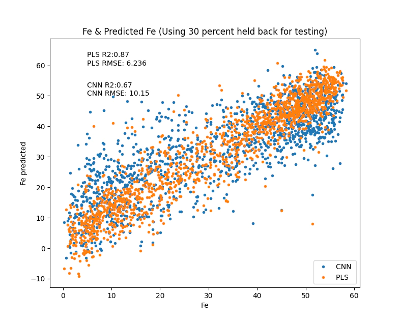
But before we go and jump straight to CNNs we train a little PLS model as a baseline.
from sklearn.model_selection import train_test_split

# before we can train a model we are going to slice out the training and testing data
borehole_info = nir.scalars[['Borehole ID', 'Depth from', 'Depth to']]
idx_borehole = borehole_info['Depth from']<0
borehole_info.loc[idx_borehole,['Depth from','Depth to']] = None
borehole_info.rename(columns={'Borehole ID':'Hole_ID'},inplace=True)

# clean up to ensure that we have the right data with out numbers that
# will cause issues later on nans negatives nulls
idx_finite_x = np.all(np.isfinite(nir.spectra),1)
idx_pos_y = scalars['Fe %']>0
idx_finite_y = np.isfinite(scalars['Fe %'])
idx_mask = scalars['Final Mask'] == 1
idx_final = idx_mask & idx_finite_x & idx_finite_y & idx_pos_y

# find the position of these indicies
pos_ok = np.where(idx_final)[0]
# seperate into test and train splits
train, test = train_test_split(pos_ok,test_size=0.3)

# simple baseline model PLS
pls_model = PLSRegression(30).fit(nir.spectra[train,:], scalars.loc[train,'Fe %'])
fehat = pls_model.predict(nir.spectra)
# very simple code to make a nice plot of our predicted values
def make_fitting_plot(x, y,meth='',location=(0,0)):
    r2 = r2_score(x, y)
    rmse = mean_squared_error(x,y, squared=False)
    fit_string = '{0}R2:{1:.2}\n{0}RMSE: {2:.4}'.format(meth, r2, rmse)
    # make a plot
    plt.plot(x,y,'.',label=meth)
    plt.xlabel('Fe')
    plt.ylabel('Fe predicted')
    plt.title('Fe & Predicted Fe (Using 30 percent held back for testing)')
    plt.text(*location, fit_string)

# just plot it
plt.figure()
make_fitting_plot(scalars.loc[test,'Fe %'],fehat[test],'PLS ',(5, 60))
plt.legend(loc = 'lower right')
plt.show()
Note how quickly the PLS model trained, we could very easily tune the number of parameters to get a more optimal model but I will leave that for now.
Moving onto CNNs I hope that you have a GPU on board, using the pretrained model here takes about 20minutes to train on CPU.
import tensorflow as tf
import tensorflow_hub as hub
# get a pre-trained model
model_url = "https://tfhub.dev/google/imagenet/efficientnet_v2_imagenet21k_ft1k_b0/feature_vector/2"
module = hub.KerasLayer(model_url,trainable=False)
# these are the magical cropping numbers that slice the chip images
crop = (( 0,0),(461,388))
model = tf.keras.Sequential([
    tf.keras.layers.InputLayer((234, 1388,3)), # take an input image
    tf.keras.layers.Cropping2D(crop), # crop to the expect shape that the pretrained model expects
    tf.keras.layers.Resizing(224,224),
    module,
    tf.keras.layers.Dense(1,activation='linear')
])
# compile the model
model.compile(loss='mean_squared_error')

# this function is modified from here:
# https://www.tensorflow.org/tutorials/load_data/images#using_tfdata_for_finer_control
def process_path(file_path,label):
    # Load the raw data from the file as a string
    img = tf.io.read_file(file_path)
    # decode the jpeg
    img = tf.io.decode_jpeg(img, channels=3)
    # resize the image and divide by 255 to get the values between 0 and 1
    # otherwise this will cause issues with the processing
    img = tf.image.resize(img, [234, 1388])/255
    return img, label

# create the dataset using tf data for the training set
dataset = tf.data.Dataset.from_tensor_slices((scalars.jpg[train], scalars['Fe %'][train]))
dataset = dataset.map(process_path)
batched = dataset.batch(32)

model.fit(batched,epochs=1,shuffle=True)

# create the test set
test_dataset = tf.data.Dataset.from_tensor_slices((scalars.jpg[test], scalars['Fe %'][test]))
test_dataset = test_dataset.map(process_path)
test_batched = test_dataset.batch(32)
# predict
cnn_yhat = model.predict(test_batched)

# and plot the results
plt.figure()
make_fitting_plot(scalars['Fe %'][test],cnn_yhat,'CNN ',(5,50))
make_fitting_plot(scalars.loc[test,'Fe %'],fehat[test],'PLS ',(5, 60))
plt.legend(loc = 'lower right')
plt.show()
With that you now have a trained model that you can apply to your data to get an Fe prediction from NIR/SWIR and chip images.
Thanks,
Ben.