too many colours
- 6 minutes read - 1167 wordsContents
I want to continue a thought chain that I had here in the last article on the logging of colour.
I was wondering how many colour codes do you need and what does a logged colour of red, green or blue actually represent?
This analysis uses all the hylogger data across Australia from the NVCL, this for the most part is diamond core in weathered material and consists of 3734 drillholes and chips. Additionally 534 Western Australian drillholes have had colour logging data extracted from WAMEX and used to compare logged to measured colour.
Before you go to far if you are not familiar with the lab colour space you can familiarise yourself with some concepts on wikipedia
Processing
Processing used a colour matching function as per the previous article on colour from hyperspectral.
Only spectra where the final mask was on was used and a subsample was taken from each hole.
Subsample selection was applied on a per hole basis and reduced the data to approximately 0.5% of the total, a schematic of the data reduction is shown in the figure below, the full data set is in red and the coloured points are the subsample.
The subsampling approach was a combination of a convex hull to ensure that the boundaries of the colour space were sampled and histogram binning to ensure approximately equal sampling across the colour space.
Random sampling did not sample the space evenly and Kmeans with stratified sampling was far too slow for a reasonable solution.
The image below is included as a representative application of the subsampling process.
All Colours
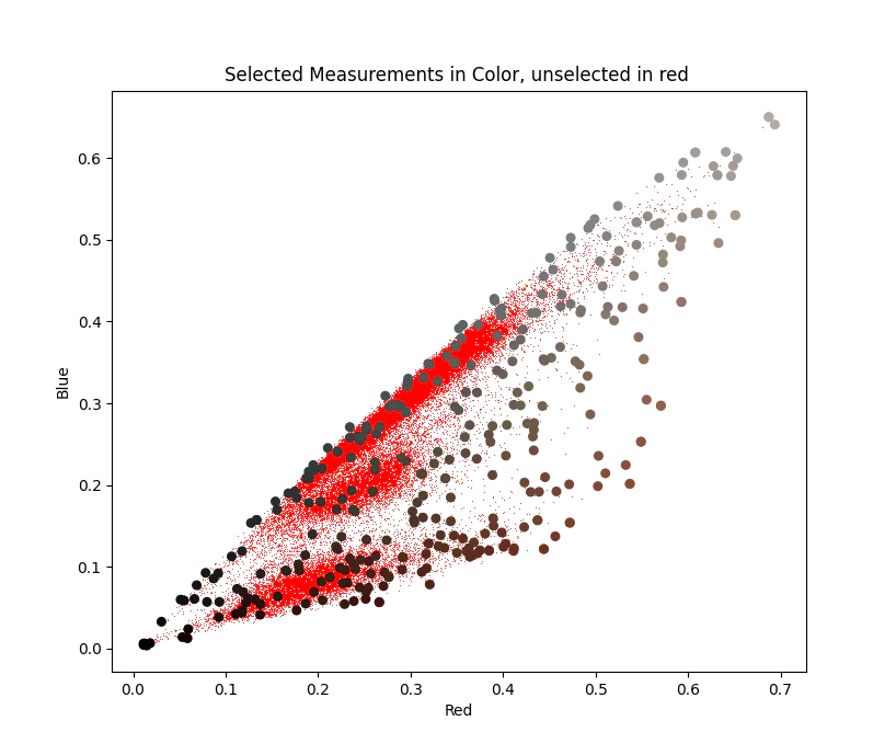
With the subsample selection complete let’s display all the colours in LAB space from the NVCL Hylogger collection.
This is the spectra from 3734 drill holes across the continent orginally consisting of 145,936,065 spectra downsampled to 735,179 spectra or a 99.5% reduction.
We can see a few interesting features where certain colours spray off into the blues and purples which is absolutely not what I expected.
Simplification
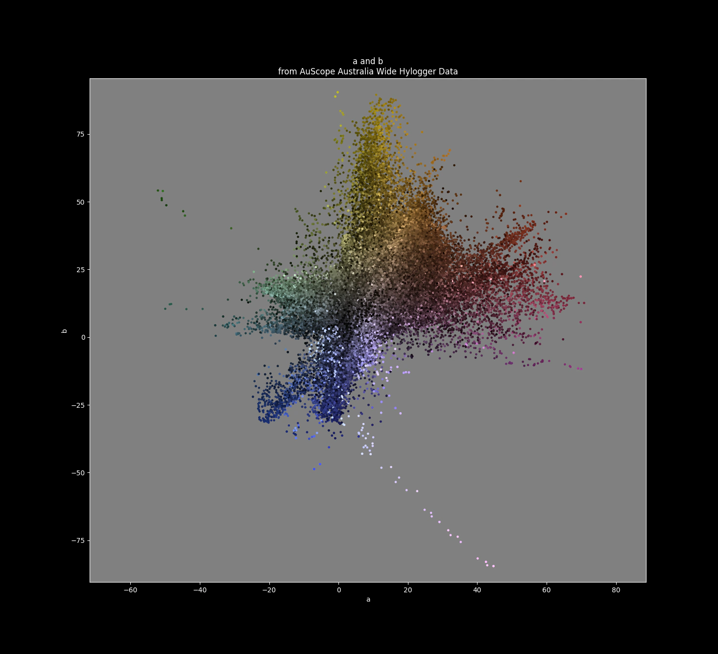
As an initial attempt at simplification we attempt to map all the measured data to their closest named colours from the xkcd colour survey dataset.
This process leaves us with 468 named colours which you can see in this diagram
So when you see someone log shit brown (not to be confused with poo brown) you know exactly the colour they are talking about.
468 named colours is too many to have for a set of logging codes we need to cut it down to a smaller set of codes.
One obvious option is to simply grid the data, but to do so we need to have a guestimate of grid size which is determined by how precisely human logging is at determining colour.
For this we will use the logged data from W.A. to attempt to detemine the accuracy and precision of manual logging.
Logging Data Comparison
To allow a comparison between the logged colour and the measured I’ve extracted the logging data from the WAMEX database for each of the hylogger drillholes in W.A. and from the logging table extracted any column that started with ‘col’. In the case of multiple columns I concatenated them together so col_1, col_2, col_3 would be concatenated to a single column.
This leaves us with a lot of colour codes that are difficult to convert to a colour, luckily 14 drill holes were logged with Munsell colour notation.
From these 14 holes we have 2917 samples where we can estimate the accuracy of the colour logging against the hylogger with the caveat that munsell chips are quite difficult to use across a large interval.
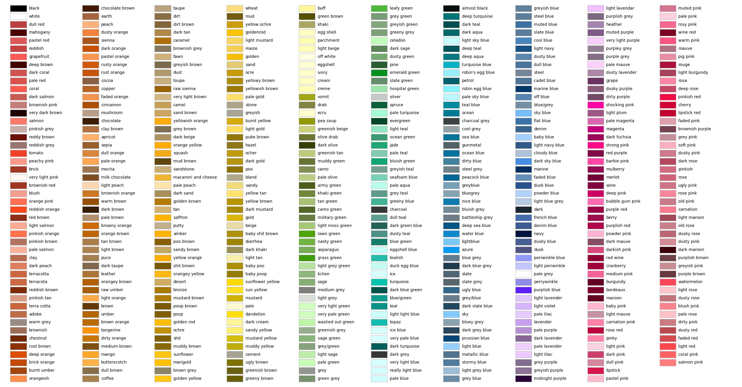
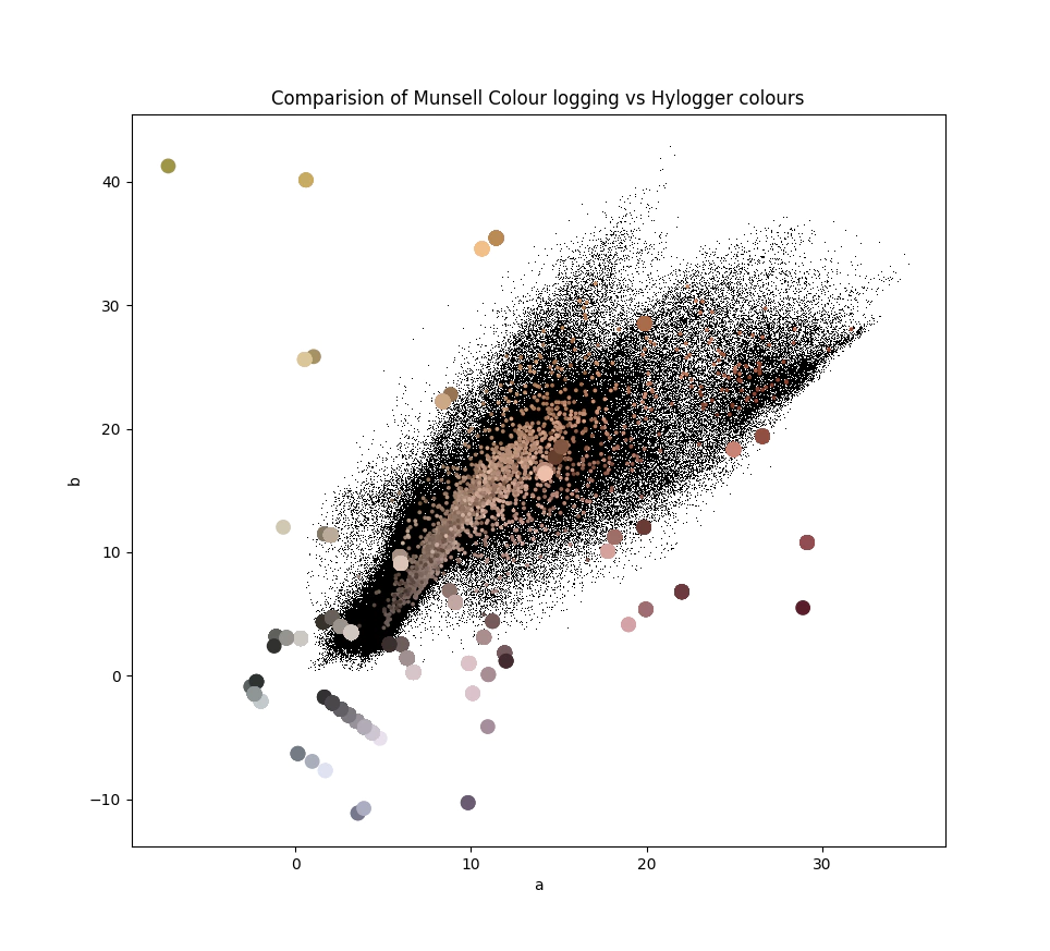
The image below plots the measured a and b parameters for both the logged munsell colours in the large coloured circles, the measured hylogger averages in the small coloured circles, the black points represent the colour of each 8mm spectral measurement.
An interesting to note is that the point measures do not reach the same colours as have been logged by the munsell chips.
Accuracy of Munsell Colour logging
To determine what level of accuracy is practially acheivable let’s look at a histogram of delta e between hylogger and human.
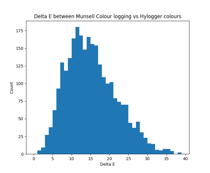
Mean delta e is around 15 which is well above the threshold for noticable colour differences according to this website.
Tolerable difference
To estimate how much difference in colour will trigger a new code being logged we are going to compare the difference in measured colour for sequential pairs of logged intervals.
There are two cases the first is where both intervals have the same colour code in the second the pair has a different code.
With the data paired by logged code we then use the hylogger measured colour to assess difference in colour for the interval.
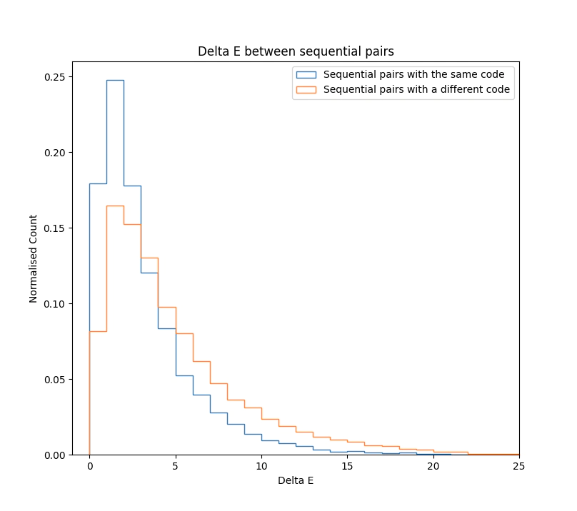
The plot above shows a slightly larger delta e for pairs where the codes are different vs the same codes. I interpret this as the logging being very inconsistent.
Consistency
To finalise we’ll run a similar analysis to the previous work on colour. where we use the hylogger colour to predict the logged colour in an attempt to assess the consistency of the prediction. This analysis uses naive bayes to generate a model classifiying logged colour from measured using this model we predict what the logged colour should be.
Perfect consistency would have a score of 1 perfect inconsistency would have a score of 0.
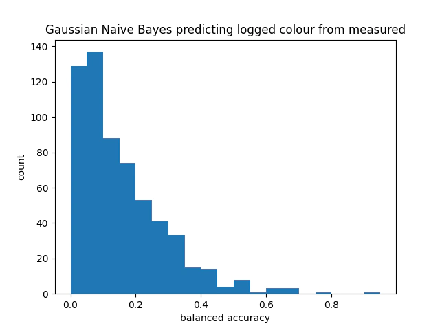
The score here is inline with the rest of the analysis, quite poor.
Codes
Moving back to simplifying the colours of AuScope using the knowledge that the accuracy of human logging is around 15 delta e we will create a grid with centres that are approximately 15 delta e apart.
For context here is a slice of the hylogger colours with an L value of between 40 and 60 this approximates the maximum saturation of colours.
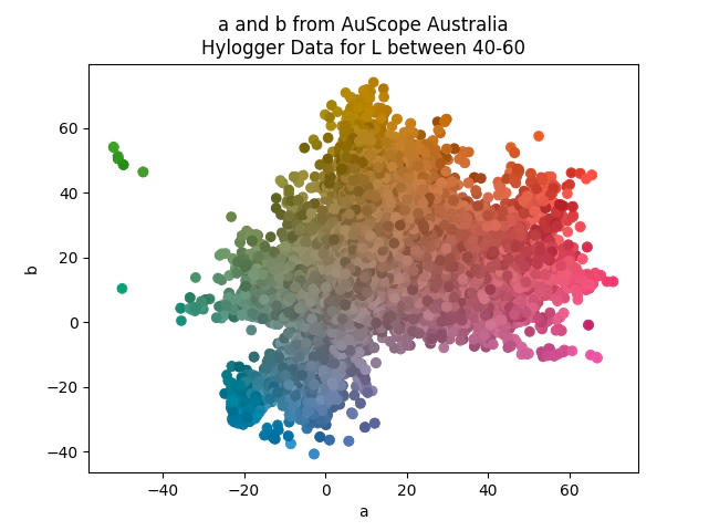
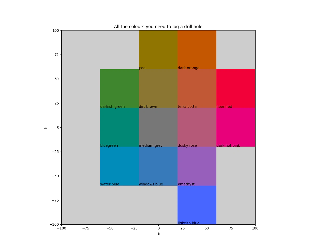
If we create a grid across this space with centres that are spaced approximately 15 delta e apart with a fixed luminance of 50 and only include grid cells that contain at least one point. We are left with this set of 14 colours that should be more than enough to log any drill hole.
Finally if you don’t like anything I’ve done you can use the data provided for the wamex drill holes with hylogger colours.
WAMEX Colours © 2023 by Ben Chi is licensed under CC BY-SA 4.0
Bonus as it’s useful but doesn’t fit in the rest of the material.
Geological Gamut
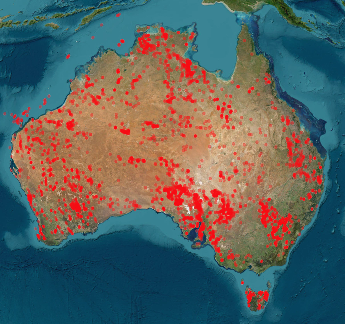
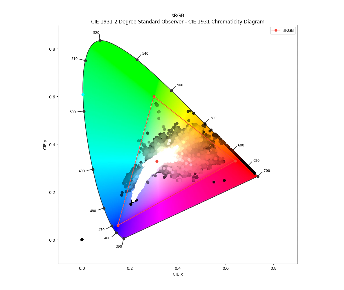
As an aside the below image shows all the subsampled data against the sRGB gamut in red, anything plotting outside the boundaries of the triangle cannot be displayed on a standard monitor.
Approximately 90% of the data sits inside the red triangle.
References
Huntington, J. (2016): Uncovering the mineralogy of the Australian Continent: the AuScope National Virtual Core Library. A national hyperspectrally derived drill-core archive.- AJES, 63 (8), 923-928
Delta E 101: http://zschuessler.github.io/DeltaE/learn/