classification of stratigraphy with hyperspectral data
- 8 minutes read - 1629 wordsLogging stratigraphy on a drill rig to decide to continue or end the hole is a skill that every geologist should have. Ideally logging happens at the rig in realtime as we are often wanting to determine end of hole critera.
Let’s consider how well hyperspectral and image data perform in classifing samples into prospective and non-prospective units.
As usual we are going to use this dataset from from the C3DMM project. To add a little something interesting we will pull from the DMIRS DASC and extract the openfile company lithological data.
Contents
- Configure Python
- Download Hyperspectral
- Download Lithology
- Parse DMP format data
- Read the TSG files
- Clean the input data
- Simplify the stratigraphy
- Datasciencing
- References
Configure Python
Let’s begin as we normally do by setting up our python install.
pip install pip install pytsg
pip install git+https://github.com/FractalGeoAnalytics/AuGeoscienceDataSets
pip install matplotlib numpy tensorflow tensorflow_hub pandas scikit-learn
Download Hyperspectral
Once we have the required libraries the next step is to download the datasets that we require. If you’ve followed the steps in the last episode you will already have the data that we need from C3DMM. If not run the section below, which will download the .tsg file pairs that you need.
from pathlib import Path
import shutil
import numpy as np
from augeosciencedatasets import downloaders
from augeosciencedatasets import readers
import pandas as pd
from matplotlib import pyplot as plt

# download the data from the csiro dap
base_dir = Path('data/')
url =  'https://data.csiro.au/dap/ws/v2/collections/44783v1/data'
target_files = ['RC_data.bip','RC_data.tsg','RC_data_cras.bip','Rocklea_Assay_MMX.xlsx']
downloaders.from_csiro_dap(url, base_dir, target_files)

# configure the path locations of the data
inputfolder = base_dir.joinpath('drill hole data/RC_hyperspectral_geochem')
tsg_file = inputfolder.joinpath('RC_data.tsg')
bip_file = inputfolder.joinpath('RC_data.bip')
cras_file = inputfolder.joinpath('RC_data_cras.bip')
image_folder= inputfolder.joinpath('img')
Download Lithological Data
Once we have the data from C3DMM the next step is to add the openfile company lithological data, which we download below.
# download the lithology data from DMIRS
outpath = Path('data/drill hole data/drillcore geochem')
dasc_url = "https://geodocsget.dmirs.wa.gov.au/api/GeoDocsGet?filekey=1924d54a-0602-49d1-b091-d1cc2739d1df-dwan6c3oozt44ggnn0y2pnp0h2xl0vrd5ybidgk4"
outfile = outpath.joinpath('A096772_drill_15042574.zip')
downloaders.from_dasc(dasc_url,outfile)

# unzip the zip file
shutil.unpack_archive(outfile,outpath)
Parse the DMP File
Now we parse the downloaded dataset from the DMP, which comes in an special format of it’s own. I have wrapped the code to do that in a package on github.
So with this file parser at hand we can read in the lithology file that we have previously downloaded and upzipped .
# parse the DMP formatted lithology data
lithology_path = Path(outpath).joinpath('Rocklea_Lithology.txt')
lithology,_ = readers.dmp(lithology_path)
Read TSG files
# read the spectra
from pytsg.parse_tsg import extract_chips, read_tsg_bip_pair

nir = read_tsg_bip_pair(tsg_file, bip_file,'nir')
# extract the images from the cras file
extract_chips(cras_file,image_folder,nir)

# add the image files to scalars
scalars = nir.scalars.copy()
scalars['jpg'] = ''
for i in Path(image_folder).glob('*.jpg'):
    idx_pair = scalars.Index.astype(int) == int(i.stem)
    scalars.loc[idx_pair,'jpg'] = i
Clean and merge the data
When creating datasets from scratch a simple process such as merging files together has a few more steps that we really want.
Because the column names for Borehole ID, Depth From and Depth To are not consistent we have to rename them.
# dictionary mapping the names in the lithology dataframe to those in the hyperspectral dataset.
lithology_columns_to_rename = {'holeid':'Borehole ID','from':'Depth from','to':'Depth to'}
# rename so that we can merge the dataframes
lithology.rename(columns =lithology_columns_to_rename,inplace=True)
# also make sure that we we have all the borehole id's in uppercase for both the hylogger and the lithology
nir.scalars['Borehole ID'] = nir.scalars['Borehole ID'].str.upper()

# make sure that we have the same datatypes
nir.scalars['Depth to'] = nir.scalars['Depth to'].astype(float)
nir.scalars['Depth from'] = nir.scalars['Depth from'].astype(float)

nir.scalars['Borehole ID'] = nir.scalars['Borehole ID'].astype(str)

lithology['Depth from'] = lithology['Depth from'].astype(float)
lithology['Depth to'] = lithology['Depth to'].astype(float)
lithology['Borehole ID'] = lithology['Borehole ID'].astype(str)
lithology['Borehole ID'] = lithology['Borehole ID'].str.upper()
Once the columns have been renamed and we have consistent datatypes we can finally merge the datasets together.
merged_data = pd.merge(nir.scalars, lithology,on=list(lithology_columns_to_rename.values()),how='left')
# convert here from an object to a category data type just to
# simplify for later on
merged_data['Strat1'] = merged_data['Strat1'].astype('category')
Simplify the Stratigraphy
There are too many strat units to deal with for this short example. So we are going to simplify the data into prospective and non-prospective units which are Archean Basement vs all else (Quaternary sediments and Cenzoic Pisolites).
# we will simplify the codes into two classes which are effectively basement and non-basement.
strat_map = {'QC':'C' ,'Czk':'C', 'Czl':'C', 'Czp':'C',  'clay':'C', 'shale':'A','AFh':'A', 'AFo':'A', np.NaN:'','Granite':'A','':''}
merged_data['Strat2'] = pd.Categorical(merged_data.Strat1.map(strat_map),categories=['C','A'],ordered=True)
Now we are ready to datascience.
Datasciencing
With our new datascience ready dataset we are finally in a position to start doing useful work.
But before jumping to something fancy-er (CNN) we need to set a baseline. As a start we are going to use sklearn and decision trees, let’s use a variation of the method outlined here and use a feature extraction to classification pipeline.
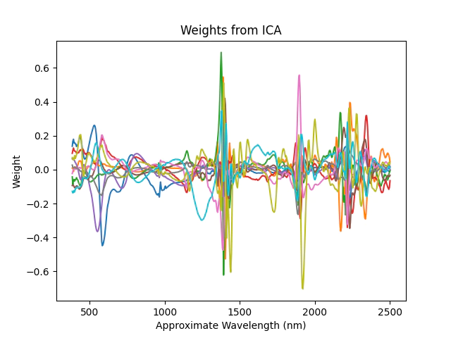
However rather than using NMF we are going to use FastICA as it is fast and returns good looking components .

from sklearn.decomposition import FastICA
from sklearn.preprocessing import FunctionTransformer
from sklearn.pipeline import Pipeline
from sklearn.ensemble import GradientBoostingClassifier
from sklearn.model_selection import train_test_split
# before we can start classifying samples we need to clean up the data
# removing nan values bad spectra and 2 samples where that cause issues when
idx_borehole = merged_data['Depth from']<0
merged_data.loc[idx_borehole,['Depth from','Depth to']] = None
idx_finite_x = np.all(np.isfinite(nir.spectra),1)
classified_y = merged_data['Strat2'].cat.codes>=0

idx_mask = merged_data['Final Mask'] == 1
idx_final = idx_mask & idx_finite_x & classified_y

# find the position of these indicies
pos_ok = np.where(idx_final)[0]
strat_ok = merged_data['Strat2'][pos_ok]
# seperate into test and train splits
X = nir.spectra[pos_ok]
Y = merged_data['Strat2'][pos_ok]
trainX, testX, trainY, testY = train_test_split(X, Y,test_size=0.3,stratify=strat_ok)

# create a function transformer to difference the spectra before using fastica
# using convex hulls are possible but are slow relatively
# differencing here is to roughly centre the data on zero which makes fastica much happier
ft = FunctionTransformer(np.diff)
# create a pipeline this just manages all the
# steps in the model building and evaluation process
pipe = Pipeline([('differ',ft), ('fica',FastICA(10)),('fitter',GradientBoostingClassifier())])
# train the model
pipe.fit(trainX,trainY)
# plot from the trained model
# and look at the weights from ICA
plt.plot(nir.wavelength[1:], pipe[1].components_.T)
plt.xlabel('Approximate Wavelength (nm)')
plt.ylabel('Weight')
plt.title('Weights from ICA')
plt.show()
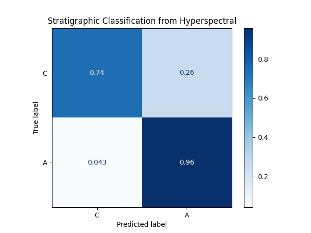
Let’s check the performance with a confusion matrix:
from matplotlib import cm
from sklearn.metrics import ConfusionMatrixDisplay
u_categories = trainY.unique()
nu_categories = len(u_categories)
ConfusionMatrixDisplay.from_estimator(
                                    pipe,
                                    testX,
                                    testY,
                                    display_labels=u_categories,
                                    cmap=cm.Blues,
                                    normalize='true',
                                )
plt.title("Stratigraphic Classification from Hyperspectral")
plt.show()

Ideally we would have only results on the diagonal. Tuning the hyperparameters would improve performance a bit, that is beyond the scope of this post.
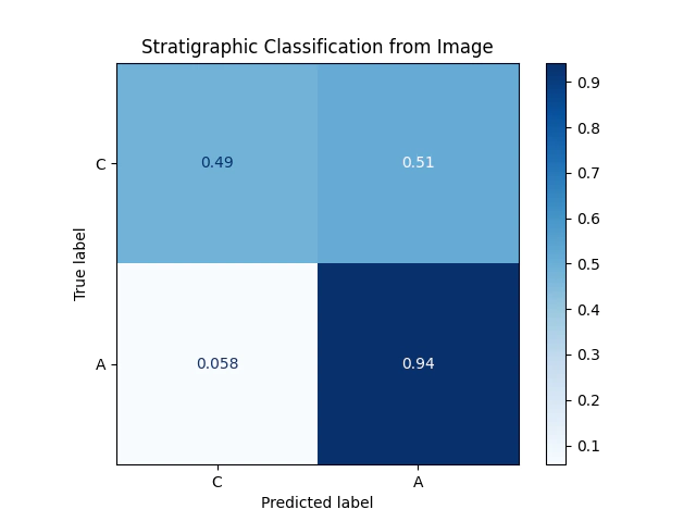
With that as a starting point, let’s check the performance using the imagery alone. Before we can train a model on the images we need to extract features from the model.
Using a pre-trained model from tensorflow hub makes this easy. This time we are going to use the vectors and a Boosted trees model to train our stratigraphic classifier rather than the neural network we trained here.
from skimage.transform import resize
import tensorflow_hub as hub
import simplejpeg
from sklearn.decomposition import PCA
# pair the extracted chip images and the rest of the information
merged_data['jpg'] = ''
for i in Path(image_folder).glob('*.jpg'):
    idx_pair = merged_data.Index.astype(int) == int(i.stem)
    merged_data.loc[idx_pair,'jpg'] = i

# get a pre-trained model
model_url = "https://tfhub.dev/google/imagenet/efficientnet_v2_imagenet21k_ft1k_b0/feature_vector/2"
module = hub.KerasLayer(model_url,trainable=False)
# let's use the pretrained model as a feature extractor similar to how we used ica to
# extract components from the NIR spectral data
# we will pre-allocate an array and place all the features into that
r = merged_data.shape[0]
c = 1280 # the hub module extracts 1280 features from the images
# we will read in batches as it is much faster to process the files
# make an range
r_index = np.arange(r)
# if you crash the program set batch to a smaller number
batch_size = 64
# calculate the number of batches
batches = np.ceil(r/batch_size).astype(int)
# preallocate an array
feature_array = np.zeros((r, c))
# loop over each of the indicies all the while reinserting the
# results into the array of features
for biter, indicies in enumerate(np.array_split(r_index,batches)):
    nimage = indicies.shape[0]
    im_array = np.zeros((nimage, 224, 224, 3))
    for i, jpg in enumerate(merged_data.jpg[indicies]):
        with open(jpg,'rb') as f:
            jbytes= f.read()
            img = simplejpeg.decode_jpeg(jbytes)
            # crop the image
            img = img[:,461:849,:]
            # resize it to the same shape that
            # the feature vector model expects
            img = resize(img,(224, 224,3))
        print('.',end='',flush=True)
        im_array[i,:,:,:] = img
    print(f'Completed:{biter} of {batches}',end='',flush=True)
    print('')
    feature_array[indicies,:] = module(im_array).numpy()
We can now pass these extracted features to a pipeline, to shorten processing time I have swapped the FastICA step with PCA.
pipe2 = Pipeline([('fica',PCA(30)),('fitter',GradientBoostingClassifier())])
# from the pandas dataframe use the index to select the correct rows of the features extracted using the cnn
train_index = trainY.index.values
pipe2.fit(feature_array[train_index], trainY)

Comparing the two confusion matricies we can see that the performance of the classifier using the images is not quite as good as the hyperspectral alone.
Of course imagery has the advantage of being quick and cheap to collect.
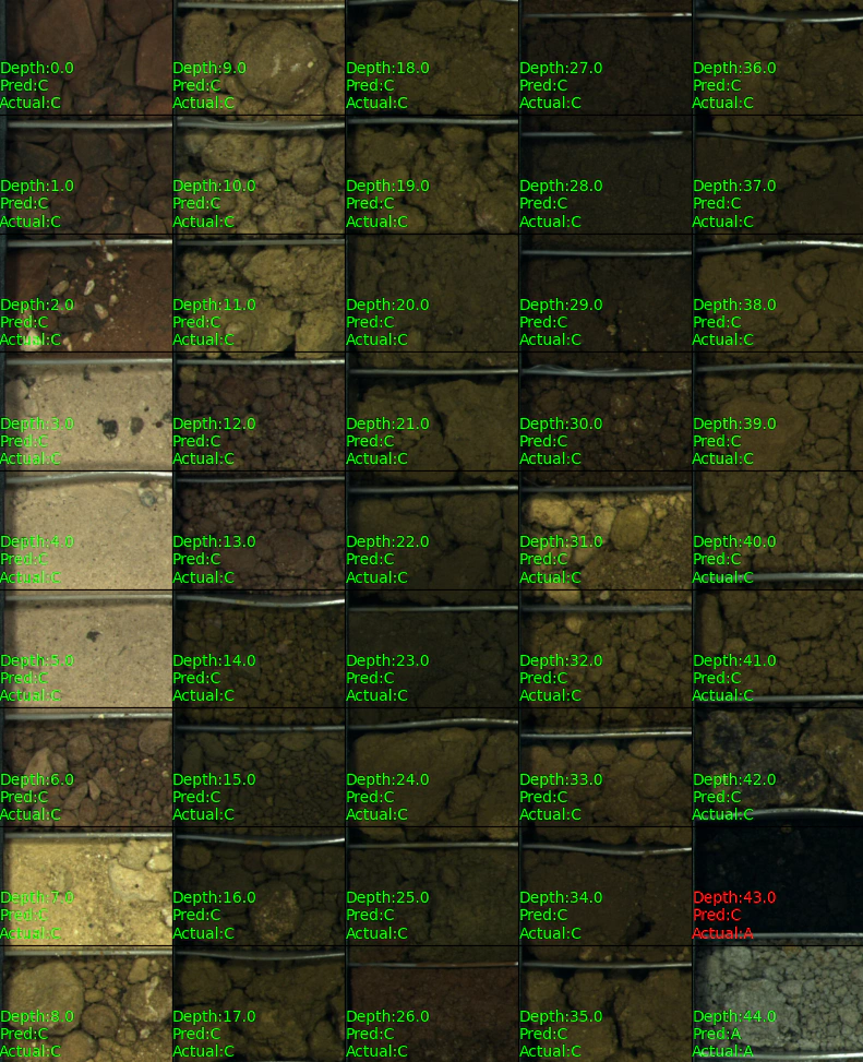
To finish up here is an example prediction on a drill hole:

# for demonstration purposes let's process a short hole from the data set.

idx = merged_data['Borehole ID'] == 'RKC485'
idx_bhid = idx[idx].index.values

nimage = idx_bhid.shape[0]

im_array = np.zeros((nimage, 224, 224, 3))
for i, jpg in enumerate(merged_data.jpg[idx_bhid]):
    with open(jpg,'rb') as f:
        jbytes= f.read()
        img = simplejpeg.decode_jpeg(jbytes)
        # crop the image
        img = img[:,461:849,:]
        # resize it to the same shape that
        # the feature vector model expects
        img = resize(img,(224, 224,3))
    im_array[i,:,:,:] = img

test_features = module(im_array).numpy()
pred = pipe2.predict(test_features)
actual = merged_data.Strat2[idx_bhid].values
depth =merged_data['Depth from'][idx_bhid].values
# a little trickery to get the subplots filled down the rows
plot_index = np.arange(nimage).reshape((9,5)).T.ravel()+1
for i in range(nimage):
    plt.subplot(9,5,plot_index[i])
    plt.imshow(im_array[i])
    plt.axis('tight')
    plt.xticks([])
    plt.yticks([])
    text = f'Depth:{depth[i]}\nPred:{pred[i]}\nActual:{actual[i]}'
    if pred[i] == actual[i]:
        text_color = [0,1,0]
    else:
        text_color = [1,0,0]
    plt.text(0, 211,text,color=text_color)
plt.subplots_adjust(wspace=0, hspace=0)
plt.show()
Thanks,
Ben.
References
Rodger, A.; Laukamp, C. Quantitative Geochemical Prediction from Spectral Measurements and Its Application to Spatially Dispersed Spectral Data. Appl. Sci. 2022, 12, 282. https://doi.org/10.3390/app12010282
Laukamp, Carsten (2020): Rocklea Dome C3DMM. v1. CSIRO. Data Collection. https://doi.org/10.25919/5ed83bf55be6a